A system design interview guide to unifying the three pillars — metrics, logs, and traces — into one platform that ingests, correlates, and queries telemetry across a fleet, replacing a pile of fragmented legacy monitoring tools.
Student edition · start with the guarantee
Unify metrics, logs, and traces through shared context while budgeting storage, coverage, and query isolation.
Correctness contract: Every signal has an explicit loss/retention policy. Correlation is configured; sampling/redaction and access controls apply before any exposed or retained sensitive copy.
Basic HTTP, databases, and programming are assumed. Specialized terms are explained below. Named products motivate the problem; this is an educational design, not a claim about their current internals. Capacity numbers are illustrative decimal payload estimates, not benchmarks. Add indexes, protocol overhead, replicas, headroom, and failure capacity before provisioning.
Most organizations grow their monitoring by accretion: a metrics system here, a log aggregator there, a tracing tool bolted on later, each with its own agents, storage, query language, and dashboards. The result is that during an incident an engineer hops between three tools that cannot talk to each other, manually copying timestamps and IDs to correlate what happened. A unified observability platform fixes this by collecting all three signal types through one pipeline, storing each in a backend suited to its shape, and — the key move — stitching them together with shared identifiers so you can pivot from a metric spike to the exact trace to the exact logs in a couple of clicks. This guide builds that platform: the pillars and their data model, a single collection layer built on OpenTelemetry, per-signal storage, the correlation glue, and the hard problems of high cardinality, multi-tenancy, and cost.
Each definition includes a concrete example and the condition under which the mechanism is useful. You can read this guide without opening another guide.
Spans and trace context
A span records one operation with a trace ID, span ID, parent or links, timing, and attributes. Context propagation sends the current trace/span identity across HTTP, RPC, thread, and queue boundaries so related work can be assembled.
Example. A gateway starts a trace, injects W3C traceparent into a service call, and the service links its queue consumer work to the producer span.
Limit. Cross-host wall clocks can skew timelines. A parent-child graph is not always a tree because asynchronous work can have multiple links. Instrumentation must be configured; IDs are not automatically present in every log.
Head and tail sampling
Head sampling decides at trace start. Tail sampling buffers received spans and decides after a configured decision interval using observed errors/latency. Sampling reduces retained volume but introduces coverage and bias choices.
Example. A 1% head sampler forwards only one in 100 traces. A later tail sampler cannot recover an error trace that the head stage never sent.
Limit. No tail policy guarantees all errors when input spans are lost, dropped, late, or evicted. Route compatible trace state together, bound memory, and report coverage before drawing aggregate conclusions.
Cardinality
The number of distinct identities a store must track. A metric series is its metric name plus the full label combination. The product of label-value counts is an upper bound when not every combination occurs.
Example. 100 hosts × 20 routes × 5 status codes can produce up to 10,000 series. Adding a unique request_id can make every request create a new series.
Limit. Hashing every ID to a distinct digest does not reduce cardinality or guarantee anonymity. Use bounded categories, explicit limits, or intentional fixed-bucket aggregation.
Inverted indexes and columnar storage
An inverted index maps searchable terms to document postings. A columnar file groups values by column so analytical scans can read only selected fields. They optimize different access patterns.
Example. 'ERROR' → document IDs {2,7}; 'service=api' → {1,2,7}. Intersection returns {2,7}. A monthly count may instead scan only time, service, and status columns.
Limit. Tokenization affects meaning, indexes have storage/write cost, and incomplete shard responses must be marked. Search refresh is visibility, not the same as durable commit.
Rollups and weighted aggregation
A precomputed summary per time bucket. Sums and counts merge by addition, min/max by comparison. An average is derived as total sum divided by total count, not an unweighted average of bucket averages.
Example. One window has [10], another [20,20,20]. Merge sum=70 and count=4 to get 17.5, not the unweighted mean of window means (10+20)/2=15.
Limit. Do not sum cumulative counter snapshots to compute traffic, or average p99 values to get a global p99. Retain reset-aware counter increases or compatible histogram distributions.
Backpressure and load shedding
Backpressure tells an upstream producer that the downstream stage cannot accept more work. Buffering delays that signal; shedding deliberately rejects or drops lower-priority work when a bound is reached.
Example. A sink accepts 100 events/s while input is 150/s. A 1000-event queue fills in 20 seconds. The system must then block, reject, or apply its documented drop policy.
Limit. A finite queue cannot absorb an infinite outage. Prioritized messages still need hard quotas, deadlines, and bounded client queues; otherwise an exemption can exhaust the system.
SLIs, SLOs, and error budgets
An SLI measures a user-relevant outcome; an SLO sets its target over a window. For a success-ratio SLO, the allowed bad fraction is 1−SLO. An SLA is a contractual commitment that may use different definitions.
Example. 99.9% successful requests over 1 billion requests allows 1 million bad requests. A time-based 30-day availability target instead allows 43.2 unavailable minutes.
Limit. Request and time budgets are not interchangeable under variable traffic or partial failure. SLOs are not universally stricter than SLAs; choose both from their definitions and user needs.
1. Requirements & Scope
Intuition
Think of a hospital. Metrics are the heart-rate monitor: one number, always on, cheap. Logs are the nurse’s notes: rich detail, lots of paper. Traces are the patient’s path through every ward. A good hospital links all three with one patient ID. An observability platform does the same with a trace_id.
Clarifying questions to ask
How many hosts, services and requests per second? (This sets every number below.)
Which signals are in scope: metrics, logs, traces, or all three? Profiles too?
Retention per signal? Hot for days, cold for months or years?
Is it multi-tenant? Do teams need quotas and isolation?
What is the alerting latency target? Seconds or minutes?
Build on OpenTelemetry, or must we support legacy agents too?
The goal is one platform that answers the three questions an operator asks during an incident: is something wrong? (metrics), what exactly happened? (logs), and where in the request path? (traces). Scope it as functional and non-functional requirements.
Functional. Ingest metrics, logs, and traces from every service and host; store each with an appropriate retention; expose query, dashboards, and alerting over all three; and let a user pivot between signals via shared context.
Vendor-neutral collection. One instrumentation standard (OpenTelemetry) so applications are not coupled to a backend and signals arrive in a common format.
Scale. Millions of metric series, terabytes of logs per day, and a firehose of spans — with ingest that never blocks the applications producing telemetry.
Query latency. Dashboards and alert evaluations return in well under a second on recent data; ad-hoc historical queries in seconds.
Multi-tenancy & cost. Many teams share the platform with isolation and quotas, and the whole thing must be affordable — telemetry volume routinely rivals the size of the production traffic it observes.
Interview tip: The single sentence that shows seniority here is “the three pillars are not three products — they are three views of the same events, and the platform’s value is the correlation between them.” Anyone can list metrics, logs, and traces; the unification is the design.
2. Back-of-the-Envelope Estimates
Sizing tells you where the money and the engineering go. Assume a mid-large fleet of 10,000 hosts running 50,000 service instances, serving 1,000,000 requests/second at peak.
Signal
Estimate
Volume math
Metrics
~20M active series; ~20M samples/s at 1s scrape
50k instances × ~400 series each ≈ 20M series; each emitted per second.
Metrics storage
~3.5 TB/day compressed (~230 GB/day at a 15 s scrape)
20M samples/s × 86,400s × ~2 bytes/sample (Gorilla-style) ≈ 3.5×10¹² B. Most fleets scrape every 15 s, which cuts this 15×; downsampled tiers keep years cheaply.
100k spans/s × 86,400s × ~1–2 KB/span ≈ 8.6–17 TB; unsampled it would be 100× more, so sampling is what makes this affordable.
Worked estimate, step by step
Step
Math
Result
Active series
50,000 instances × 400 series
20M series
Metric samples
20M series ÷ 1 s scrape
20M samples/s
Metric bytes/day
20M × 86,400 s × 2 B
≈ 3.5 TB
Log bytes/s
1M req/s × 10 lines × 500 B
5 GB/s
Log bytes/day (raw)
5 GB/s × 86,400 s
≈ 432 TB
Kept spans/day
100k spans/s × 86,400 s × 1–2 KB
≈ 8.6–17 TB
Raw ingest per day
3.5 + 432 + ~13
≈ 450 TB/day (logs ≈ 96%)
Read the table
Logs are almost all of the bytes. So log tiering and log compression are where the money goes. Metrics are tiny by comparison.
The estimate immediately explains three design decisions: metrics compress fantastically and are cheap to keep, so they are the always-on layer; logs are the bulk of raw bytes, so tiering and cheap object storage dominate their design; and traces are so voluminous raw that sampling is mandatory, not optional. Each pillar therefore gets a different storage strategy.
3. The Three Pillars & Data Model
Each pillar answers a different question and has a different data shape, which is precisely why one storage engine cannot serve all three well.
Metrics. Numeric measurements aggregated over time — request rate, error rate, p99 latency, CPU. Cheap, always on, low-dimensional. Identified by a name plus a set of key-value labels; the name-plus-labels defines one time series. Great for “is something wrong and how much?” but they tell you nothing about an individual request.
Logs. Discrete, timestamped event records, ideally structured (JSON) with fields. High volume, high detail. Great for “what exactly happened?” on a specific event, at the cost of being expensive to store and search at scale.
Traces. The causal record of one request as it flows across services — a tree of spans, each a timed unit of work with a trace_id, span_id, and parent link. Great for “where did the latency go?” across a distributed call path.
The unifying thread is context: every signal carries a common set of resource attributes (service, host, region) and, wherever it originates inside a request, the trace_id and span_id. That shared context is what later lets the platform join a metric, a log, and a trace that describe the same moment.
4. API & Data Model
Apps never call the stores directly. They speak OTLP to a collector. Users speak a query API to one front end.
# write path (OTLP over gRPC or HTTP)
POST /v1/metrics   ResourceMetrics{ resource{service,host}, points[ {name, labels, ts, value, exemplar?} ] }
POST /v1/logs      ResourceLogs{ resource, records[ {ts, severity, body, attrs, trace_id?, span_id?} ] }
POST /v1/traces    ResourceSpans{ resource, spans[ {trace_id, span_id, parent_id, name, start, end, attrs, status} ] }

# read path (one query layer over three stores)
GET /api/metrics/query_range?q=<PromQL>&start&end&step
GET /api/logs/search?q=<LogQL/Lucene>&start&end&limit
GET /api/traces/{trace_id}
GET /api/traces/search?service&min_duration&status=error
POST /api/alerts/rules   { expr, for, labels, receivers }
The one field that ties it all together is trace_id. It rides on spans, on log records, and on metric exemplars.
5. High-Level Architecture
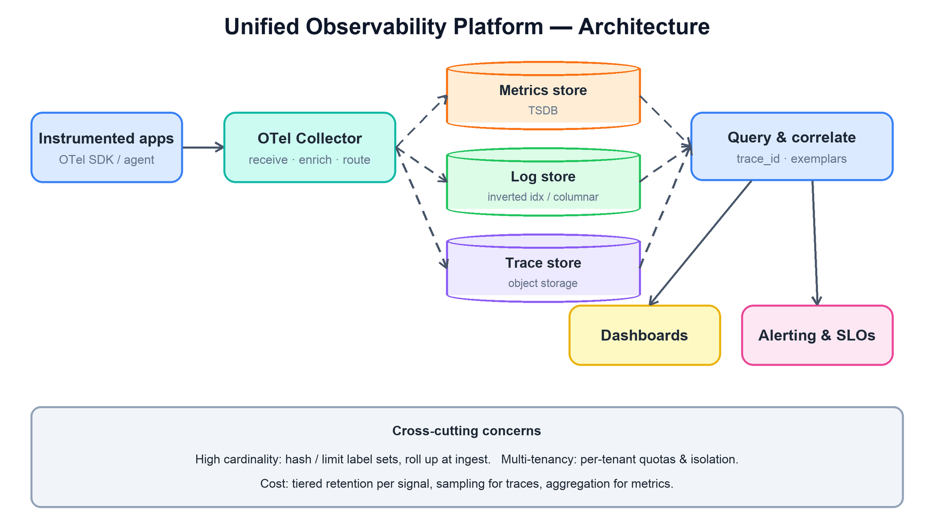
The platform is a pipeline: instrument once, collect through one layer, route each signal to its own store, and query and alert over all of them with a correlation layer on top.
Applications are instrumented with the OpenTelemetry SDK and emit all three signals to a collector, which receives, enriches, and routes each signal to a purpose-built store — a TSDB for metrics, an inverted-index or columnar store for logs, and an object-storage-backed trace store. A query-and-correlate layer serves dashboards and alerting, and cross-cutting concerns (cardinality, tenancy, cost) apply at every stage.
The design deliberately splits collection from storage from query. Collection is a common front door so applications never know or care which backend stores their telemetry. Storage is specialized per signal because their access patterns differ so sharply. And the query layer sits above all three stores so a single UI can correlate them. This separation is exactly what a fragmented legacy setup lacks — there, each tool owns its own collection, storage, and query, and nothing joins across them.
6. Collection & OpenTelemetry Ingest
OTel SDKs instrument operations and export signals; context propagation and log injection must be configured in supported frameworks or manually. A collector pipeline has signal-specific receivers, processors, and exporters; a compact list here is conceptual, not valid copy-and-run YAML.
Run agents for local collection and gateways for tenant policy/routing and eligible tail sampling. Bound SDK/collector queues, memory, disk, retry, and export time. Decide drop versus backpressure per signal; audit data may need a different durable path. Redact sensitive fields before any retained transport/archive/DLQ required by policy. Tail sampling cannot restore head-discarded or lost traces.
7. Storage Per Signal
Each pillar gets a store matched to its shape. Forcing all three into one engine is the classic mistake that makes a platform either slow or ruinously expensive.
Metrics → time-series database
Metrics are stored in a TSDB optimized for append-heavy writes and range-scan reads over (timestamp, value) pairs. It uses an inverted index on labels to select series, delta-of-delta timestamp and XOR value compression to shrink the data dramatically, and downsampling into coarser resolutions as data ages so years of history stay cheap. (See the companion time-series store guide for the internals.)
Logs → inverted index and/or columnar
Logs need full-text and field search, so they go into an inverted index (Lucene-style, as in Elasticsearch/OpenSearch) for recent data, and increasingly into a columnar format (Parquet on object storage) for older data and analytical scans. Indexing every field is expensive, so a cost-conscious design indexes a few high-value fields and stores the rest as compressed columns queried by scan. (See the companion log search guide.)
Traces → key-by-trace_id store
Spans are written keyed by trace_id so that all spans of a request can be fetched together to reassemble the trace. Because span volume is enormous, the store is backed by cheap object storage with a small index from trace_id (and searchable attributes) to the blocks that hold its spans — the model used by systems like Grafana Tempo. (See the companion distributed tracing guide.)
8. Correlation via Trace IDs & Exemplars
Correlation is the whole point of unifying the pillars, and it works because every signal carries shared context. Two mechanisms tie them together.
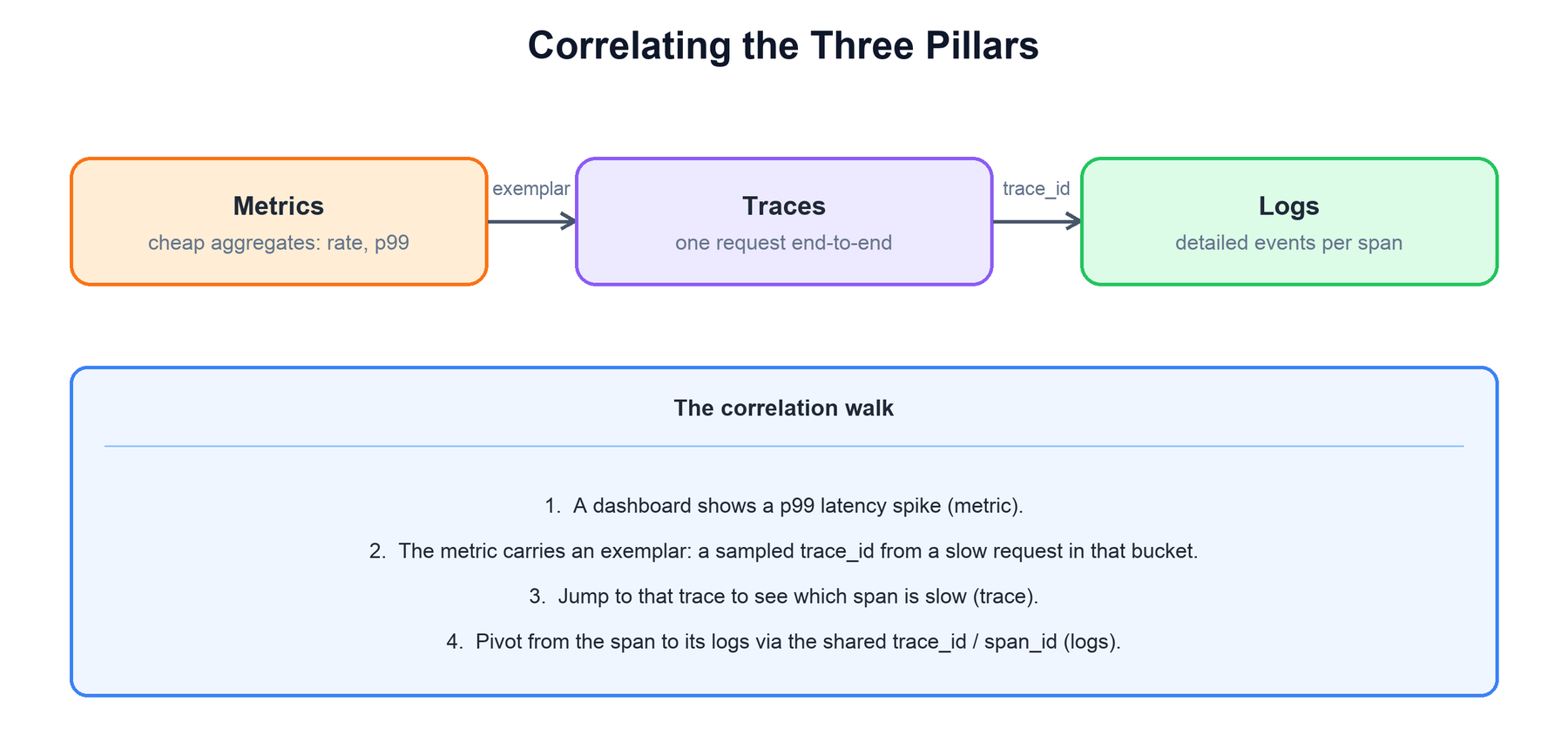
From a metric spike, an exemplar — a sampled trace_id attached to a metric bucket — jumps you to a representative slow trace; from a span in that trace, the shared trace_id and span_id pivot you to the exact logs. The three pillars become one investigation.
Exemplars (metrics → traces). A metric aggregate like a latency histogram loses per-request detail by design. An exemplar attaches a sample trace_id to a histogram bucket, so when a dashboard shows a p99 spike you can click straight through to an actual slow trace that landed in that bucket — bridging the aggregate world of metrics and the individual world of traces.
Trace/span IDs (traces ↔ logs). Because the OTel SDK injects the current trace_id and span_id into every log line emitted during a request, you can pivot from any span to exactly the logs it produced, and from any log line back to its trace. This is the join key that turns three silos into one graph.
The investigation flow this enables — metric spike → exemplar → slow trace → span logs — is what an interviewer is really testing when they ask you to “unify” observability. Shared, propagated context is the mechanism; a common query layer over all three stores is what surfaces it.
9. Cardinality, Multi-Tenancy & Cost
Metrics cardinality is observed label combinations. Hashing distinct unbounded IDs into distinct digests does not reduce it; hashing can also leave identities reversible through dictionary attacks. Use curated bounded labels, fixed buckets only with intentional semantics, and per-tenant series/churn limits.
Logs/traces also need bounded attributes/indexing cost, retention, authentication, access checks, query fairness, and ingest quotas. Sampling reduces coverage and can bias investigation/aggregates; expose policy and drop rates. Redact before durable brokers/archive/DLQ where the data policy requires it, not merely before one queryable sink.
Collection buffers are finite. Define behavior when memory/disk/export budgets fill, keeping production-request overhead bounded; a collector cannot promise isolation from an unbounded outage. Exemplar/trace-log correlation requires configured instrumentation and retained context, not automatic IDs in every line.
10. Failure Modes & Tradeoffs
Failure
What happens
Defense
A storage backend is slow or down
Collectors back up, then drop data
Collector queues with retry; a Kafka buffer before the stores; per-signal isolation so logs failing never blocks metrics
Cardinality explosion
TSDB memory and index blow up; queries time out
Per-tenant series limits; drop or hash unbounded labels at the collector
One tenant floods ingest
Other teams lose data or alerts
Per-tenant rate limits and quotas at the gateway
Heavy dashboard query
Query layer stalls; alerts evaluate late
Separate alert evaluation from ad-hoc queries; query timeouts and cost limits
The monitoring system itself dies
Silence looks like health
Meta-monitoring on a separate stack plus a dead-man’s-switch alert
Choice
Option A
Option B
Log storage
Full inverted index: fast search, costly
Label index + compressed chunks or columnar: cheap, slower grep
Trace sampling
Head: cheap, may miss errors
Tail: keeps errors and slow traces, needs trace-aware routing and memory
Metric resolution
1 s scrape: sharp, 15× the data
15–60 s scrape: cheap, may hide short spikes
Deployment
Agent per host: local buffering
Central gateway only: simpler, one hop more fragile
Worked example: a label hash does not solve cardinality
A service records one million distinct user IDs.
Read top to bottom. The table below explains the state and guarantee at each step.
Step
State, calculation, and reasoning
1. Count original labels
A user_id label can create one million distinct series for one metric.
2. Hash each ID
A cryptographic digest still has nearly one million distinct values. It hides representation, not cardinality, and is not necessarily anonymous.
3. Choose a bounded dimension
Aggregate by a meaningful bounded category or intentionally map to a fixed bucket count with changed semantics; keep per-user detail in a governed events/log store.
4. Correlate an investigation
An exemplar can link a histogram observation to a trace only if the SDK/config captured and retained it. Log injection and trace coverage are not automatic.
Check your understanding: Does an OTel collector guarantee no application slowdown during any backend outage?
No. Memory/disk queues are finite and exporter SDK policies vary. Choose bounded buffering/drop/backpressure and expose loss.
Run a small, testable model
Download concepts.py. It uses only the Python 3.10+ standard library. From the directory where you saved it, run:
python3 concepts.py observability
python3 concepts.py test
The model checks label-cardinality preservation and sampling limits, then prints SLO budget arithmetic.
The program contains deterministic assertions and failure traces. It is a learning model, not a production service: it does not implement network consensus, distributed durability, authentication, or third-party delivery. Read its contracts and try changing an input before extending it.
Ask the clarifying questions. Pin fleet size, signals, retention and tenancy.
5–10
Run the estimate. Point out that logs dominate bytes and traces need sampling.
10–20
Draw SDK → agent → gateway → three stores → query layer. Name OTLP.
20–30
Deep dive one store the interviewer cares about. Metrics TSDB or log tiering is common.
30–38
Show correlation: exemplar → trace → logs by trace_id.
38–45
Cardinality, multi-tenancy, cost, and who monitors the monitor.
12. Common Mistakes
Watch out
Putting all three signals in one database. Their access patterns differ too much.
Using a user id or request id as a metric label. That is a cardinality bomb.
Keeping 100% of traces. The bytes are 100× the sampled volume.
Forgetting to put trace_id in log lines. Without it there is no correlation.
Running alerting on the same cluster it watches, with no dead-man’s switch.
13. Summary
A unified observability platform collects all three signals through one standard pipeline, stores each in a backend matched to its shape, and — the differentiator — correlates them with shared context so investigation is one flow instead of three.
Concern
Mechanism
What are the pillars?
Metrics (is it broken?), logs (what happened?), traces (where in the path?) — three views of the same events.
TSDB for metrics, inverted-index/columnar for logs, key-by-trace_id object store for traces.
How do the pillars connect?
Exemplars link metrics → traces; shared trace_id/span_id link traces ↔ logs.
What breaks it at scale?
High cardinality — bound labels, drop/hash at ingest, enforce per-series limits.
How do many teams share it?
Per-tenant quotas, isolation, and fair query scheduling.
How do we afford it?
Tiered retention, downsampling, trace sampling, index only high-value fields.
The recurring theme: unify at the edges (one instrumentation standard, one collection pipeline, one query layer) but specialize in the middle (a store per signal). The value is not the three pillars individually — it is the shared, propagated context that lets you walk from a metric to a trace to a log describing the same event.
14. Check Yourself
Why do logs dominate the storage bill in this design?Answer
Each request makes about 10 lines of 500 B. That is 5 GB/s, or about 432 TB/day raw. Metrics are about 3.5 TB/day and kept traces about 13 TB/day.
What is an exemplar and what problem does it solve?Answer
It is a sample trace_id attached to a metric bucket. A histogram loses per-request detail. The exemplar lets you click from a p99 spike to a real slow trace.
Why does tail sampling need a gateway tier?Answer
The keep-or-drop choice needs every span of a trace. Spans come from many hosts. A gateway routes by trace_id so one node sees the whole trace.
A team adds user_id as a metric label. What breaks, and how do you stop it?Answer
Each user makes a new series. The TSDB index and memory blow up. Stop it with per-tenant series limits and a collector rule that drops or hashes the label.
Why use OpenTelemetry instead of each vendor’s agent?Answer
Apps instrument once against one API and wire format. You can then swap or fan out backends without touching app code.
How do you know the monitoring system itself is healthy?Answer
Run meta-monitoring on a separate stack. Add a dead-man’s-switch alert that fires when the expected heartbeat stops.
15. Key Terms
Metric
A number over time, keyed by name and labels.
Series
One unique name + label set. The unit of TSDB cost.
Cardinality
The number of distinct identities a store must track. A metric series is its metric name plus the full label combination. The product of label-value counts is an upper bound when not every combination occurs. Example and limits above.
Span
A span records one operation with a trace ID, span ID, parent or links, timing, and attributes. Context propagation sends the current trace/span identity across HTTP, RPC, thread, and queue boundaries so related work can be assembled. Example and limits above.
Trace
The tree of spans for one request.
Exemplar
A sample trace_id stored on a metric bucket.
OTLP
OpenTelemetry’s wire protocol for all three signals.