A system design interview guide to building an operational metrics store — the kind that ingests millions of data points per second, keeps years of history without going broke, and answers a dashboard query in milliseconds.
Student edition · start with the guarantee
Store timestamped metric series while preserving the meaning of counters, gauges, and aggregated distributions.
Correctness contract: A series identity is stable; writes have an explicit durable/ordering policy; rollups retain enough information for the queries they promise.
Basic HTTP, databases, and programming are assumed. Specialized terms are explained below. Named products motivate the problem; this is an educational design, not a claim about their current internals. Capacity numbers are illustrative decimal payload estimates, not benchmarks. Add indexes, protocol overhead, replicas, headroom, and failure capacity before provisioning.
Every large system is wired with sensors: counters for requests served, gauges for memory used, timers for latency, one metric for almost everything an operator might want to graph. Collected together at scale, these emit an astonishing firehose of timestamped numbers, and somebody has to store them in a way that is cheap to write, cheap to keep, and fast to query. A general-purpose database struggles with this workload because it was not built for it — the access pattern is overwhelmingly append-only writes and range-scan reads over a very specific shape of data. A purpose-built time-series store, of the sort an operational data store like ODS provides, makes a handful of specialized choices that a relational database cannot. This guide builds up those choices: the data model, the write path, downsampling into retention tiers, the compression tricks that make years of history affordable, and the query path that ties it together.
Each definition includes a concrete example and the condition under which the mechanism is useful. You can read this guide without opening another guide.
Cardinality
The number of distinct identities a store must track. A metric series is its metric name plus the full label combination. The product of label-value counts is an upper bound when not every combination occurs.
Example. 100 hosts × 20 routes × 5 status codes can produce up to 10,000 series. Adding a unique request_id can make every request create a new series.
Limit. Hashing every ID to a distinct digest does not reduce cardinality or guarantee anonymity. Use bounded categories, explicit limits, or intentional fixed-bucket aggregation.
Rollups and weighted aggregation
A precomputed summary per time bucket. Sums and counts merge by addition, min/max by comparison. An average is derived as total sum divided by total count, not an unweighted average of bucket averages.
Example. One window has [10], another [20,20,20]. Merge sum=70 and count=4 to get 17.5, not the unweighted mean of window means (10+20)/2=15.
Limit. Do not sum cumulative counter snapshots to compute traffic, or average p99 values to get a global p99. Retain reset-aware counter increases or compatible histogram distributions.
Write-ahead log and fsync
A WAL records updates before data pages are considered committed. Recovery replays it after a crash. fsync (or an equivalent storage contract) requests that buffered bytes reach durable storage rather than only process/OS memory.
Example. A server acknowledges after its WAL commit and required replica writes are durably accepted. A process crash can then reconstruct the committed update.
Limit. Appending to a file alone does not guarantee power-loss durability. Device behavior, filesystem ordering, replicas, corruption, and the declared fault budget still matter.
Inverted indexes and columnar storage
An inverted index maps searchable terms to document postings. A columnar file groups values by column so analytical scans can read only selected fields. They optimize different access patterns.
Example. 'ERROR' → document IDs {2,7}; 'service=api' → {1,2,7}. Intersection returns {2,7}. A monthly count may instead scan only time, service, and status columns.
Limit. Tokenization affects meaning, indexes have storage/write cost, and incomplete shard responses must be marked. Search refresh is visibility, not the same as durable commit.
Event time and watermarks
Event time is when the producer says an event happened; processing time is when a consumer handles it. A watermark is the processor's policy-driven estimate of event-time progress, used to emit and eventually clean up window state.
Example. An event for 12:00 arrives at 12:07. A 5-minute allowed-lateness policy may update its window, divert it to correction, or reject it according to the API contract.
Limit. Watermarks are not proof all earlier events arrived. Idle inputs, skew, and unbounded delay require explicit policies; later corrections must propagate to rollups and reports.
Offsets and checkpoints
An offset is a position in one log partition. A checkpoint is a recoverable, consistent record of input positions and processing state. On restart, state must correspond exactly to the input that is considered processed.
Example. If a batch increments a total and crashes before saving its offset, replay increments twice. Commit the total, dedup state, and partition position together, or use a compatible transactional/idempotent sink.
Limit. Saving an offset after a write avoids that specific loss window but can still duplicate; framework checkpoints alone do not make arbitrary external effects transactional.
1. Requirements and Clarifying Questions
What is being stored? Infrastructure and app metrics, not logs or traces. (Assume numeric metrics only.)
How many series? (Assume 10,000 hosts × 500 series each = 5 M active series.)
How often? (Assume one point every 10 s per series.)
Who queries? Dashboards and alert rules. Alerts run every 15–60 s and must not miss.
How long? (Assume raw 15 days; rollups for 90 days, 2 years, and 5 years.)
Functional
Non-functional
Write points (name, tags, ts, value).
Sustain 500 K points/s; never block writers on reads.
Query by metric, tag filter, and time range with aggregation.
Dashboard queries under 1 s over the last few hours.
Support counters (rate) and gauges.
Alert evaluation keeps working during query storms.
Downsample and expire old data automatically.
Years of history at low cost.
2. Back-of-the-Envelope Estimation
Illustrative inputs: 5 million active series sampled every 10 seconds produce 500,000 points/s and 43.2 billion points/day. Sixteen payload bytes per point give 691.2 GB/day before indexes, framing, replicas, and storage overhead. Gorilla's paper reports about 1.37 bytes/point on its measured workload; applying that as a hypothesis gives 59.2 GB/day, not a universal bound.
Rollup storage depends on the actual fields and measured encoded size. For four 8-byte aggregates, 5-minute payloads alone are 5M×288×32≈46.1 GB/day before compression/metadata. Measure count/sum/min/max separately and add retained tiers, index/head memory, WAL, churn, compaction space, replicas, and failure headroom. Five million series can fit on some fleets, but arithmetic payload size alone does not prove a few servers meet the workload.
3. The Data Model
The whole design rests on a deliberately narrow data model. A single data point is the combination of four things, and pinning them down early is what lets every later layer be specialized.
Metric name. What is being measured, for example http.requests or cpu.usage. It names the series family.
Tags / labels. A set of key-value pairs that identify which instance of that metric, for example host=web42, region=us-east, status=200. The metric name plus its full set of tags defines a single, distinct time series.
Timestamp. When the measurement was taken, usually at second or millisecond resolution.
Value. The number itself — a floating-point reading.
So a data point is (name, {tags}, timestamp, value), and a series is the ordered sequence of (timestamp, value) pairs that share one name-and-tags identity. This is the unit everything operates on: writes append a point to a series, reads scan a range within one or more series, and compression works down the (timestamp, value) columns of a series. The narrowness is the point — because the shape is so constrained, the storage engine can make assumptions a general database never could.
Component
Example
Role
Metric name
http.requests
Names the family of series.
Tags
host=web42, status=200
Selects one specific series within the family.
Timestamp
1700000000
Position along the time axis of that series.
Value
97.3
The measurement at that instant.
4. Counters vs Gauges
Values come in two flavors, and the distinction changes how they are queried even though they are stored the same way. Knowing which is which is the difference between a sensible graph and a meaningless one.
Gauges. A gauge is a snapshot reading that can go up or down — current memory in use, temperature, queue depth, number of active connections. You graph a gauge directly; its instantaneous value is meaningful on its own.
Counters. A counter only ever increases — total requests served, total bytes sent, total errors since the process started. The raw value of a counter is almost never interesting; what you want is its rate of change. You graph a counter by taking the difference between consecutive points and dividing by the time between them, turning "total requests" into "requests per second."
A common interview trap is treating a counter like a gauge. Plotting a raw counter shows an ever-rising line that tells you little and resets to zero whenever the process restarts. The store keeps the raw monotonic values; the query layer applies a rate function to make them useful. That function must be reset-aware: when a value drops, the process restarted, so the increase is the new value, not a negative number. Knowing where that conversion happens — read time, not write time — signals real familiarity.
A counter only goes up, except when the process restarts and it starts again from zero. A naive difference shows a huge negative spike. Reset-aware rate functions, such as Prometheus rate(), treat any drop as a restart.
5. High Cardinality
The hardest scaling problem in a metrics store is not the volume of points; it is the number of distinct series, known as cardinality. Cardinality is the product of every tag's distinct values. One metric tagged by host, status code, endpoint, and region explodes combinatorially: a thousand hosts times a hundred endpoints times a dozen status codes is already over a million distinct series from a single metric name.
Cardinality hurts because the store must track an index entry and an in-flight write buffer for every active series. A tag whose values are effectively unbounded — a user id, a request id, a raw timestamp jammed into a label — is the classic cardinality bomb: each new value mints a brand-new series forever, and the index grows without limit until memory is exhausted. The defenses are mostly disciplinary: keep tags to bounded, low-cardinality dimensions; never put unbounded identifiers in labels; and put limits and monitoring on series creation so a misbehaving client cannot take the system down by inventing millions of series.
Tag
Cardinality
Verdict
region
~10 values
Fine — bounded and small.
status
~40 values
Fine — bounded.
host
thousands
Acceptable, watch it.
user_id
millions+
Cardinality bomb — never use as a tag.
6. API and Data Model
# write (agents push batches; or the server scrapes /metrics endpoints)
POST /api/v1/write
  [{ "name": "http_requests_total",
     "labels": { "service": "checkout", "status": "500", "host": "web42" },
     "samples": [[1758808987000, 18234], [1758808997000, 18251]] }]

# query: errors per second by service over the last hour, 1-minute steps
GET /api/v1/query_range?query=sum by (service) (rate(http_requests_total{status="500"}[5m]))
                       &start=-1h&end=now&step=60s
Immutable files for older data; merged by compaction.
Rollup blocks
(series_id, resolution, window)
sum, count, min, max (and last for gauges).
7. The Write Path
The write path is engineered around one fact: the workload is overwhelmingly appends. Points arrive in roughly time order, almost always newer than what came before, and are rarely updated once written. That lets the ingestion path be far simpler and faster than a general database's.
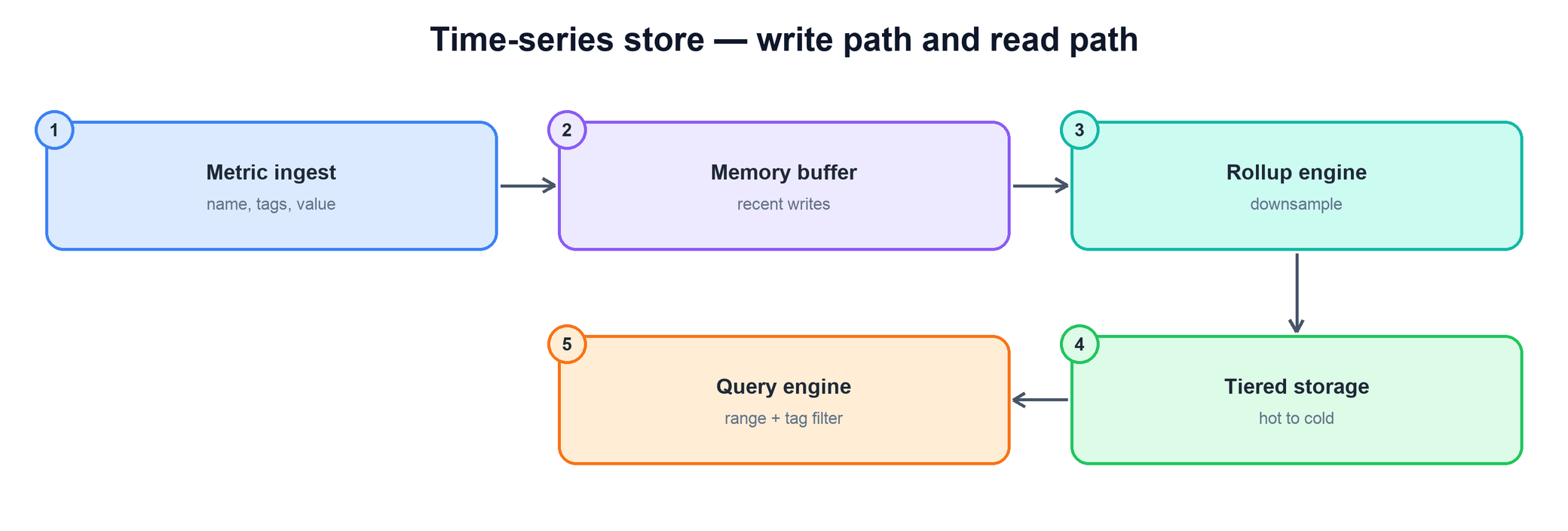
Incoming points are resolved to a series, logged to the WAL and appended to an in-memory head block. Full blocks are flushed to disk at full detail. A background compactor later downsamples old raw blocks into rollups. The query engine reads the head block, raw blocks and rollups and merges them by time.
The stages:
Metric ingest. Receivers accept batches of (name, tags, timestamp, value) points from agents running on every host. They resolve each point to its series id and route it onward. This layer is stateless and scales horizontally with the write load.
Memory buffer. Recent points for each active series are held in an in-memory structure — the hot, write-optimized tier. Appending to an in-memory column is far cheaper than a disk write per point, and because reads of "the last few minutes" are the most common dashboard query, keeping recent data in memory serves them instantly. The buffer is backed by a write-ahead log so a crash does not lose unflushed points.
Flush and rollup. When a block of the buffer is complete (say two hours of data), it is compressed and flushed to disk at full resolution. A separate background job (often called compaction) later reads those raw blocks and writes the coarser rollup tiers (covered next). Raw data is never thrown away at flush time; it expires later by retention.
Tiered storage. Flushed, compressed blocks land in durable storage organized from hot (recent, high-resolution, fast media) to cold (old, low-resolution, cheap media).
Query engine. Reads fan out across the memory buffer and the storage tiers, stitching together recent and historical data to answer a query.
function write(point):
  series_id = index.resolve(point.name, point.tags)  # name + tags -> series
  wal.append(series_id, point.ts, point.value)       # durability first
  buffer[series_id].append(point.ts, point.value)    # hot in-memory append
  if buffer[series_id].block_complete():
    flush(compress(buffer[series_id]))                # raw, compressed block

function compactor():                                 # background, off the write path
  for block in raw_blocks_older_than(ROLLUP_AGE):
    write_rollup(downsample(block, "5m"))             # sum, count, min, max per window
8. Rollups and Retention Tiers
Choose retention and aggregates from query requirements. For gauges, store sum, count, min, and max; combine means as total sum/total count. If you retain a fifth aggregate, name it and explain its use rather than silently assuming five two-byte values. Missing samples and uneven spacing require an explicit sample-weighted versus time-weighted policy.
For cumulative counters, sum of snapshot values is not traffic. Retain a reset-aware increase/rate representation, boundary information, and duration; take rate per original series before summing across instances so resets remain visible. A drop suggests a reset under the exporter contract, but can also be an ordering/source error.
For histograms, sum compatible bucket counts/sums or merge a documented distribution sketch, then compute a quantile. Global p99 cannot be obtained by averaging per-window or per-shard p99s. Once raw data expires, queries are restricted to retained resolution and sufficient statistics; do not promise arbitrary historical detail.
9. Compression
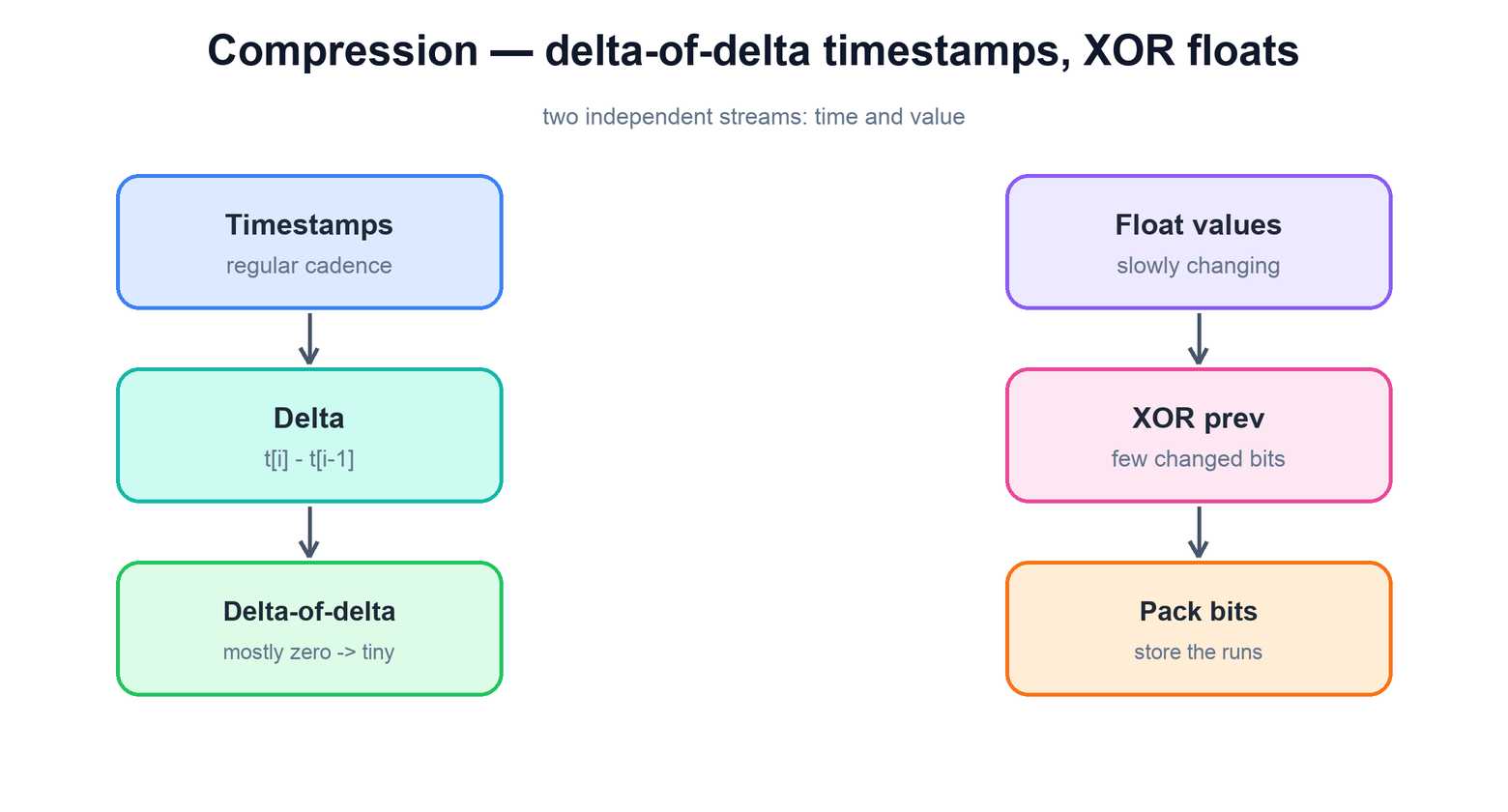
Even with rollups, the raw tier holds an enormous number of points, so compression is what makes the whole thing economical. Time-series data compresses extraordinarily well because both its columns are highly regular, and the canonical techniques — popularized by the Gorilla in-memory store — exploit that regularity directly. The trick is to compress timestamps and values as two separate streams.
Timestamps are compressed with delta-of-delta: regular cadence makes the second difference almost always zero, stored in a tiny number of bits. Values are XORed against the previous value: slowly changing floats differ in only a few bits, which are packed compactly.
Delta-of-delta on timestamps. Points usually arrive at a fixed cadence — say every minute. The difference between consecutive timestamps (the delta) is therefore nearly constant, and the difference between consecutive deltas (the delta-of-delta) is almost always zero. Storing a long run of zeros takes almost no space, so a stream of regular timestamps collapses to a handful of bits per point instead of a full 64-bit timestamp.
XOR on values. Adjacent readings of a real metric tend to be close — CPU usage at 50.1% then 50.2%. XORing each float against the previous one yields a result that is mostly zero bits, with only a small middle band of differing bits. Storing just that band of meaningful bits, rather than the whole 64-bit float, shrinks slowly-changing series dramatically. When a value is unchanged, the XOR is all zeros and costs a single bit.
# timestamps: store the second difference (usually 0)
dod[i] = (ts[i] - ts[i-1]) - (ts[i-1] - ts[i-2]) # regular cadence -> 0# values: XOR against previous, store only the changed bits
xor = bits(value[i]) ^ bits(value[i-1]) # mostly zero bits
store(leading_zeros(xor), meaningful_bits(xor)) # skip the zeros
The combined effect is striking: Facebook's Gorilla paper reports an average of about 1.37 bytes per point, against 16 bytes for a raw 64-bit timestamp plus 64-bit value — roughly 12× smaller. This is what lets the hot tier live in memory and the cold tiers stay affordable. The insight worth stating in an interview is why it works — time-series data is regular in both axes, so you store differences and changed bits rather than full values.
10. The Query Path
A query against a metrics store has a recognizable shape: it picks a metric, filters by tags, restricts to a time range, and aggregates. The engine answers it by turning that into a series selection plus a scan plus a fold.
Series selection by tags. An inverted index maps each tag key-value pair to the set of series carrying it. A filter like host=web42, status=200 intersects the matching sets to find exactly the series to read. This is what makes "show me errors across all hosts in us-east" fast instead of a full scan.
Range scan. For each selected series, the engine reads the compressed (timestamp, value) blocks overlapping the requested time window, choosing the resolution tier that fits, and decompresses them.
Aggregation. The points are folded — summed, averaged, rated for counters, or grouped across series — into the final result the dashboard plots. Order matters for counters: take the rate of each series first, then sum across series (sum(rate(x[5m]))). Summing raw counters first hides each series' resets. Grouping by a tag, for example summing request counts across all hosts per region, happens here.
function query(metric, tag_filter, start, end, agg):
  series = index.match(metric, tag_filter)     # inverted index intersection
  tier   = pick_resolution(start, end)         # finest tier covering the range
  result = []
  for s in series:
    points = storage.scan(s, tier, start, end) # decompress overlapping blocks
    result.append(aggregate(points, agg))      # avg / sum / rate / ...
  return combine(result, agg)                  # group across series
11. Read vs Write Separation
The write and read workloads have almost nothing in common, so a robust design keeps them on separate paths. Writes are a relentless, latency-sensitive append stream that must never stall; reads are spiky, often expensive range scans driven by humans opening dashboards and by alerting rules evaluating continuously. Letting a heavy read query contend with the ingest path is how a metrics system falls over exactly when an incident makes everyone open dashboards at once.
Separation shows up at several layers. The ingest tier and the query tier scale independently, so a surge of dashboard traffic does not slow ingestion and a write spike does not slow queries. The memory buffer serves recent reads directly without disturbing the flush pipeline. And because the data is immutable once flushed, historical reads can be served from the storage tiers with no coordination against ongoing writes at all — there are no locks to contend, since old blocks never change. The result is a system that keeps ingesting through a query storm and keeps serving queries through a write spike.
The theme echoes the rest of the design: specialize relentlessly. Just as the data model is narrowed so storage can make assumptions, the paths are split so each can be tuned for its own workload. A general database mixes these and pays for it; a purpose-built metrics store separates them and wins.
12. Failure Modes
Failure
What happens
Mitigation
Ingest node crashes
Head block in memory lost.
Replay the WAL on restart; run two replicas that both ingest the same series.
Cardinality explosion
Index memory grows until OOM.
Per-tenant and per-metric series limits; reject new series past the cap; alert on series churn.
Expensive query (a year of raw data)
Query nodes overload.
Query limits (samples, series, time); route long ranges to rollups; separate alerting from ad-hoc queries.
Late or out-of-order points
Rejected or placed in a closed block.
Accept a small out-of-order window in the head; drop or backfill-block anything older.
Counter reset
Negative spikes on graphs.
Reset-aware rate().
Missing scrapes (host down)
Gaps; alerts may not fire.
Alert on absence (up == 0) as well as on values.
13. Tradeoffs and Alternatives
Choice
Option A
Option B
Pick when
Collection
Pull (server scrapes targets, Prometheus)
Push (agents send, StatsD/OTLP)
Pull gives free up/down health and central control. Push suits short-lived jobs and firewalled hosts.
Columnar OLAP (ClickHouse) or general DB (TimescaleDB)
TSDB for metrics at scale; OLAP when you need high-cardinality slicing or SQL joins.
Rollup timing
At ingest (pre-aggregate)
Background compaction
Ingest-time is cheaper to query but you lose raw detail you did not plan for.
Long-term storage
Local disks
Object storage (Thanos, Cortex/Mimir)
Object storage for years of history and global queries.
High-cardinality data
Labels in the TSDB
Logs, traces, or an events store
Per-user or per-request detail belongs outside the metrics store.
Worked example: why averages and counter snapshots cannot be summed blindly
Two windows have gauge samples [10] and [20,20,20]. A process counter separately records 100,120,5,15 after a reset.
Read top to bottom. The table below explains the state and guarantee at each step.
Step
State, calculation, and reasoning
1. Compute the gauge rollup
First window: sum=10,count=1. Second: sum=60,count=3. Combined mean is 70/4=17.5, not mean(10,20)=15.
2. Detect a counter reset
Counter drops from 120 to 5. Under a reset-to-zero assumption, observed increases are 20+5+10=35, not 15−100 and not the sum of snapshots.
3. Retain query-specific state
Gauge sum/count/min/max cannot reconstruct arbitrary raw samples. Counter rates need reset-aware increases/duration; p99 across shards needs compatible distributions, not averaged p99 values.
4. Budget active series
1000 hosts×100 routes×12 status values is an upper bound of 1.2 million combinations. Only observed combinations exist, but per-request labels can still explode state.
Check your understanding: Is Gorilla's published compression ratio a provisioning guarantee?
No. It is an observed result on one workload. Measure representative series, headers, rollup encodings, indexes, churn, replicas, and headroom before selecting a fleet.
Run a small, testable model
Download concepts.py. It uses only the Python 3.10+ standard library. From the directory where you saved it, run:
python3 concepts.py rollups
python3 concepts.py test
The model checks weighted means and reset-aware counter increases, then contrasts them with the wrong calculations.
The program contains deterministic assertions and failure traces. It is a learning model, not a production service: it does not implement network consensus, distributed durability, authentication, or third-party delivery. Read its contracts and try changing an input before extending it.
Series count, interval, query types, alerting, retention.
5–10
Estimate
500 K points/s; 59 GB/day compressed; series count drives memory.
10–15
Data model
name + labels = series; counters vs gauges; cardinality.
15–30
Write path and storage
WAL + head block, immutable blocks, Gorilla compression, compaction and rollups.
30–40
Read path
Inverted index, pick the tier, reset-aware rate, sum of rates.
40–45
Scale and failures
Shard by series hash, replicas, cardinality limits, query limits, alerting isolation.
15. Common Mistakes
Averaging averages in rollups. Store sum and count; divide on read.
Ignoring counter resets. Naive differences go negative after a restart.
Summing counters before taking the rate. Use rate per series, then sum.
Putting user ids or request ids in labels. Every new value creates a new series forever.
Downsampling at flush time. You lose raw data you may need for the next two weeks.
Letting dashboards and alerts share one query pool. An incident dashboard storm then delays alerts.
16. Summary
A metrics / time-series store is a specialist database whose every choice flows from a single observation: the data has a narrow, regular shape, and the workload is append-heavy writes with range-scan reads.
Concern
Mechanism
What is a data point?
Metric name + tags + timestamp + value; name plus tags identifies one series.
How are values interpreted?
Gauges graphed directly; counters converted to a rate at read time.
What is the dominant scaling limit?
Cardinality — keep tags bounded, never label with unbounded ids.
How do we ingest at scale?
Append-optimized path: stateless ingest, in-memory buffer with a WAL, then flush.
How do we keep years of history cheaply?
Downsample into coarser resolutions with longer retention as data ages.
How do we make storage affordable?
Delta-of-delta timestamps and XOR float compression on regular series.
How do we answer a query fast?
Inverted tag index to select series, range scan the right tier, aggregate.
How do we stay stable under load?
Separate read and write paths; immutable flushed blocks need no read-write coordination.
The recurring theme: narrow the data model so the engine can specialize, then exploit the regularity everywhere — append-only writes, downsampled tiers, differential compression, and split read/write paths. The result handles a firehose of points, keeps years of history for little money, and still answers a dashboard in milliseconds.
17. Check Yourself
A metric has labels host (2,000 values), endpoint (50), and status (8). What is the worst-case number of series?
Answer
2,000 × 50 × 8 = 800,000 series for that one metric name. In practice fewer combinations occur, but plan for the product.
A counter reads 100, then 120, then 7 (restart), then 30, at 10 s intervals. What is the total increase?
Answer
20 + 7 + 23 = 50 over 30 s, so the average rate is about 1.67/s. A naive difference would include −113 and give a negative rate.
Two 5-minute windows have averages 10 (from 30 points) and 40 (from 10 points). What is the 10-minute average?
Answer
(10×30 + 40×10) ÷ 40 = 700 ÷ 40 = 17.5. The average of averages, 25, is wrong. This is why rollups keep sum and count.
Why does delta-of-delta encoding make regular timestamps almost free?
Answer
With a fixed interval every delta is the same, so the delta-of-delta is 0. Gorilla stores a 0 in a single bit.
5 M series at a 10 s interval, 1.37 bytes per point. How much disk per day for raw data?
Answer
5 M ÷ 10 = 500 K points/s × 86,400 = 43.2 B points × 1.37 B ≈ 59 GB/day.
Why should user_id never be a label, and where should that data go instead?
Answer
Each user creates a new series, so index memory grows with the user count. Per-user detail belongs in logs, traces, or an events/OLAP store.
18. Key Terms
Series
One metric name plus one exact set of labels.
Cardinality
The number of distinct identities a store must track. A metric series is its metric name plus the full label combination. The product of label-value counts is an upper bound when not every combination occurs. Example and limits above.
Gauge
A value that can go up or down, graphed as is.
Counter
A value that only increases (until restart); graphed as a rate.
Counter reset
A counter dropping to zero when its process restarts.
Head block
In-memory recent data, backed by a WAL.
WAL
Write-ahead log: append-only file replayed after a crash.
Compaction
Background merging of blocks and writing of rollups.
Downsampling
Replacing fine points with coarser aggregates (sum, count, min, max).
Delta-of-delta
Difference between consecutive timestamp gaps; usually 0.
Postings list
Sorted series ids for one label=value; the inverted index.
Further reading
Tuomas Pelkonen et al., "Gorilla: A Fast, Scalable, In-Memory Time Series Database," VLDB 2015.
Prometheus documentation: data model, metric types, and the rate() function.
Google, Site Reliability Engineering, chapter 6 (Monitoring Distributed Systems).
Martin Kleppmann, Designing Data-Intensive Applications, chapter 3 (storage and retrieval, LSM trees, column storage).