Starting from "what is a neural network", and finishing at how a real one runs on a GPU. No prior knowledge assumed.
33 slides · ← / → to navigate, or put #N in the URL · every number and every figure here was computed, not asserted.
Traditional programming: you write the rules, the computer applies them. Machine learning: you supply examples, the computer works out the rules.
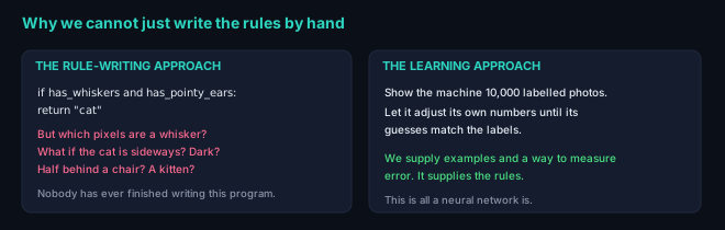
You can look at a photograph and say "cat" in about 150 milliseconds. Now try to write down the instructions. Not "it has fur" — actual instructions, in terms of the numbers a computer sees, which is all a photograph is.
Nobody has ever managed it. People tried seriously for roughly forty years.
There are no objects in an image file. There is a grid of numbers, one per pixel, each giving a brightness from 0 (black) to 255 (white). A colour photo has three such grids: red, green and blue.
A small 224 × 224 colour photo:
224 × 224 × 3 = 150,528 numbers
Your task: write a function that maps
those 150,528 numbers to "cat" or "dog".
Every idea you have will break. Move the cat two pixels left and every number changes. Turn the light down and every number changes. The cat is still a cat.
| Ingredient | What it is | In our example |
|---|---|---|
| Data | Examples with correct answers | 10,000 photos, each labelled cat or dog |
| Model | A formula with adjustable numbers | The neural network |
| Loss | A score for how wrong it is | One number, which we want small |
Training means adjusting the model's numbers until the loss is small. That is the whole idea. The next eight slides are only the details of how.
Supervised learning means every training example comes with the correct answer attached. Somebody had to label those 10,000 photos. That labelling is usually the expensive part of a real project, far more expensive than the computing.
If you understand this one picture, you understand the atom that everything else is built from.
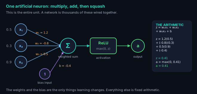
Each incoming number is multiplied by a weight. A large positive weight means "this input matters a lot, and in favour". A negative weight means "this input argues against".
The weights are the neuron's opinion. They start random and are corrected by training.
Sum all the multiplied values, then add one extra number called the bias. The bias shifts the whole result up or down, letting the neuron fire more or less readily regardless of its inputs.
Steps 1 and 2 together are just a weighted average with an offset.
Pass the sum through an activation function. Here it is ReLU: keep the number if it is positive, otherwise output zero.
This step looks trivial. The next slide shows that without it, nothing works at all.
A neuron has exactly two kinds of number: the inputs, which come from the data or from the previous layer and change with every example, and the weights and bias, which belong to the neuron and stay fixed while it is being used. Training is the process of changing the second kind. Nothing else about the network ever changes — not the structure, not the arithmetic, only those numbers.
Suppose we remove the activation function. Layer one computes y = W₁x. Layer two computes z = W₂y. Substitute:
Two layers collapse into one layer with a single combined weight matrix. Add a hundred more and they still collapse into one. A stack of straight lines is a straight line.
The activation function is the bend that stops the collapse. It is the only reason depth means anything.
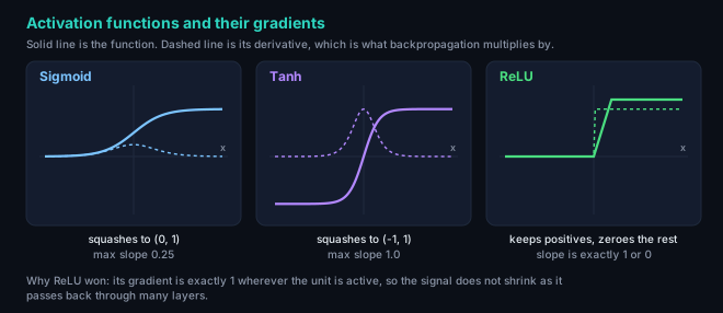
The solid line is the function: what the neuron outputs. The dashed line is its slope at each point, which is the number training uses to decide how to adjust the weights.
Look at sigmoid on the left. Away from the centre the dashed line is almost flat on the floor. A slope near zero means "adjusting this weight changes nothing", so learning stops. That is the vanishing gradient problem, and it is why deep networks were considered untrainable for years.
| Function | Output range | Use it |
|---|---|---|
| ReLU | 0 to ∞ | Everywhere inside the network. This is the default. |
| Sigmoid | 0 to 1 | Final layer only, for a yes/no answer as a probability |
| Softmax | Sums to 1 | Final layer, for choosing one of several classes |
| Tanh | −1 to 1 | Rarely; largely replaced by ReLU |
| GELU | ≈ −0.17 to ∞ | Modern large models; a smoother ReLU |
If you are unsure, use ReLU in the hidden layers and softmax at the output. That combination covers the overwhelming majority of real networks.
| Term | Meaning |
|---|---|
| Layer | A row of neurons that all read the same inputs |
| Input layer | The raw numbers; it does no computing |
| Hidden layer | Any layer in between. "Hidden" only means you do not observe it directly. |
| Output layer | The final answer: one neuron per class |
| Width | Neurons in a layer |
| Depth | Number of layers. "Deep learning" means nothing more than this. |
| Fully connected | Every neuron reads every output of the previous layer |
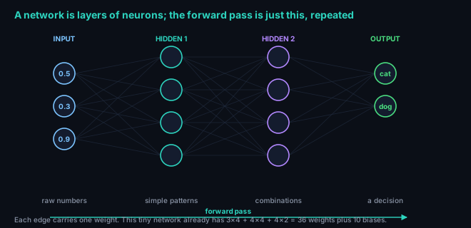
| Forward pass | Running data left to right to get a prediction |
Doing this one neuron at a time is tedious, so a whole layer is written as a matrix multiply. For a layer with weights W and biases b:
Chain three of those together and you have the entire network:
That expression is a complete neural network. Everything that follows in this deck is about choosing a better shape for W, and about how to find good values for the numbers inside it.
Layer sizes: 3 → 4 → 4 → 2 weights: 3×4 + 4×4 + 4×2 = 12 + 16 + 8 = 36 biases : 4 + 4 + 2 = 10 total = 46
Forty-six numbers to learn. A network that recognizes handwritten digits needs roughly 100,000. GPT-scale language models need hundreds of billions. The arithmetic on this slide does not change; only the size of the matrices does.
The network cannot improve until "wrong" becomes a number it can try to reduce.
Run an example through the network. Compare the prediction with the correct answer. Produce a single number: large if wrong, small if right, zero if perfect. That number is the loss.
Average it over all the training examples and you have one number describing how good the entire network currently is. Training is the search for weights that make it small.
Mean squared error — for predicting a quantity, such as a house price:
Cross-entropy — for choosing a category, which is what classification means:
Cross-entropy is worth a moment. If the network gives the right answer a probability of 1.0, the loss is −log(1) = 0: no penalty. As that probability approaches zero the loss grows without limit. It punishes confident mistakes far more harshly than uncertain ones, which is exactly the behaviour you want.
The correct answer is "cat". Here is what the loss says about three different networks:
| P(cat) | P(dog) | Verdict | Loss = −log P(cat) |
|---|---|---|---|
| 0.99 | 0.01 | right, confident | 0.01 |
| 0.70 | 0.30 | right, unsure | 0.36 |
| 0.50 | 0.50 | no opinion | 0.69 |
| 0.20 | 0.80 | wrong | 1.61 |
| 0.01 | 0.99 | wrong, confident | 4.61 |
Note the last row. Being confidently wrong costs 460 times more than being confidently right. That steep penalty is what pushes the weights hard in the right direction.
Before a network has learned anything it should guess uniformly at random. For C classes that gives each a probability of 1/C, so the starting loss should be approximately:
For 10 classes that is ln(10) = 2.303. If your training starts at 2.30, the setup is sound. If it starts at 47, something is wrong before you have trained at all, and no amount of training will repair it.
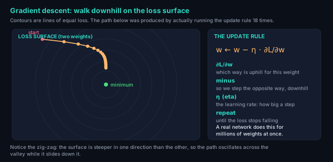
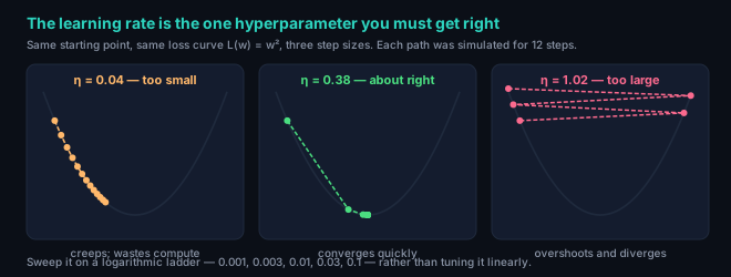
Imagine you are standing on a foggy hillside and want to reach the bottom of the valley. You cannot see the valley. But you can feel which way the ground slopes under your feet, so you take a step downhill, and repeat.
The hillside is the loss, plotted against the weights. Your position is the current set of weights. The slope you can feel is the gradient. That is the entire algorithm.
For a single weight, the gradient ∂L/∂w answers one question: if I increase this weight slightly, does the loss go up or down, and by how much?
Subtracting the gradient handles all three cases at once, which is why the update rule is a single line.
| Piece | Read it as |
|---|---|
w | One weight, out of possibly millions |
∂L/∂w | Which way is uphill for this particular weight |
− | Go the other way, because we want to descend |
η (eta) | The learning rate: how large a step to take |
← | Overwrite the old value with the new one |
Every weight in the network is updated by this same rule, independently, at every step. There is no second algorithm hiding behind it.
| Variant | Examples used per step | In practice |
|---|---|---|
| Batch GD | All of them | Accurate but far too slow |
| Stochastic GD | One | Fast but very noisy |
| Mini-batch GD | 32 to 256 | What everybody actually uses |
When somebody says "SGD" they almost always mean mini-batch. The batch size is chosen to keep the hardware busy, and 32 to 256 is the usual range.
Gradient descent needs a gradient for every weight. Backpropagation is the method that produces them all in one sweep.
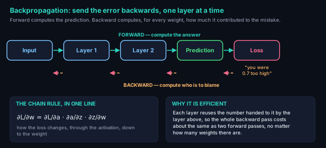
The network predicted "dog" and the answer was "cat". Some weight buried in layer two contributed to that mistake. How much? You cannot measure it directly, because that weight only affects the loss through everything downstream of it.
The naive alternative is to nudge each weight, re-run the whole network and see what changes. For a million weights that is a million forward passes per step. Completely impractical.
Start at the loss, where the error is known exactly. Ask the last layer: given this error, how much did each of your weights contribute, and how much error should I pass to the layer before you? Then ask that layer the same question. Repeat to the start.
Each layer only needs the number handed down from the layer above it, plus values it already saved during the forward pass. Nothing is recomputed from scratch.
Read right to left: how the weight affects the sum, times how the sum affects the activation, times how the activation affects the loss. Multiply the three and you have how the weight affects the loss.
This is ordinary calculus from a first course, applied mechanically. The insight in backpropagation is not the mathematics; it is the order of evaluation that lets every weight share the work.
| Method | Cost per training step |
|---|---|
| Nudge each weight and re-run | One forward pass per weight |
| Backpropagation | About two forward passes, total |
For a network with 25 million weights that is the difference between 25 million forward passes and two. Backpropagation is the reason training a large network is possible at all, and it is why the field stalled until it became widely understood in 1986.
PyTorch, TensorFlow and JAX record every operation you perform and derive the backward pass automatically. In practice you write loss.backward() and the gradients appear. It is still worth understanding, because almost every training bug you will meet is a gradient that is zero, enormous, or not flowing at all.
NaN.If your loss becomes NaN in the first few steps, the learning rate is the first thing to divide by ten.
| Term | Meaning |
|---|---|
| Batch | A handful of examples processed together, usually 32 to 256 |
| Step | One batch: forward, loss, backward, update |
| Epoch | One complete pass over the training data |
| Learning rate | Step size. Start at 0.1 for SGD, 0.001 for Adam. |
| Optimizer | The rule that applies the update. SGD and Adam are the two you need. |
| Schedule | A plan for shrinking the learning rate as training proceeds |
for epoch in range(num_epochs): for batch_x, batch_y in training_data: # 1. Forward: what does the network say? prediction = model(batch_x) # 2. Loss: how wrong is that? loss = loss_function(prediction, batch_y) # 3. Clear the gradients from last time optimizer.zero_grad() # 4. Backward: blame every weight loss.backward() # 5. Update: w ← w − η · gradient optimizer.step()
That is a complete PyTorch training loop. It is the same five steps whether the model has 46 parameters or 46 billion, and it is the same loop used to train every network in the rest of this deck.
PyTorch adds new gradients to whatever is already stored rather than replacing them. Omit zero_grad() and every batch silently accumulates on top of all previous batches. Training will not crash. It will simply behave strangely and you will not know why. This is the single most common beginner bug.
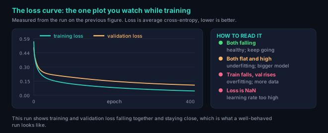
A two-layer network with 10 hidden neurons, trained by the exact loop on the previous slide. Both figures come from that one run.
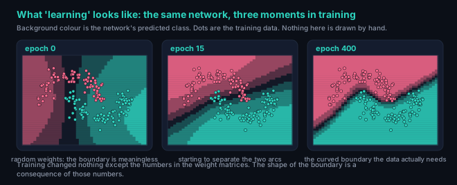
The two colours of dot are two classes that cannot be separated by a straight line. The background shading is the network's opinion at every point on the plane.
At epoch 0 the weights are random and the boundary is meaningless. By epoch 400 it has curved itself around the shape of the data. The only thing that changed is the values inside two small weight matrices.
Training loss is measured on the data the network learns from. Validation loss is measured on data it has never seen, held back deliberately. The gap between them is the single most informative thing in machine learning:
You now have the complete machinery: neurons, layers, a loss, gradients, backpropagation and a training loop. Everything in Part 2 reuses it without modification.
The next slide asks one question: what happens when we point this exact machinery at a photograph?
Take the fully connected network you just learned, point it at a photograph, and it breaks in three specific ways.
A single ImageNet image is 224 × 224 × 3 = 150,528 numbers. Connect that to one modest hidden layer of 1,000 units:
That is one layer. It already exceeds the 138M parameters of the entire VGG-16 network, and 25.6M of ResNet-50. At 4 bytes per float the layer alone is 602 MB.
A dense layer has an independent weight for every pixel position. A cat in the top-left and the same cat in the bottom-right activate two completely disjoint sets of weights.
The network must learn "cat" separately at every one of the 50,176 spatial positions. Nothing in the architecture says the two are related, so nothing transfers.
Flattening the image destroys adjacency. Pixel (10, 10) and pixel (10, 11) are neighbours; after flatten they are indices 2,250 and 2,253 with no relationship the layer can see. Permute all input pixels with a fixed permutation and a dense network trains to the same accuracy. That is the tell: it never used the spatial structure.
| Property | Dense | Conv |
|---|---|---|
| Connectivity | Global | Local (K×K) |
| Weights per output | 150,528 | 27 (3×3×3) |
| Weights reused? | No | Every position |
| Shift the input | Unrelated output | Output shifts too |
| Params scale with | Image size | Kernel & channels only |
The last row is the one that matters most. A 3×3, 3→64 conv layer has 1,792 parameters whether the input is 32×32 or 4096×4096.
These are assumptions about images, not about learning. They are why a CNN needs far less data than an unstructured model to reach the same accuracy, and why they fail on data where the assumptions do not hold, such as tabular features in arbitrary column order.
Hubel and Wiesel (1962) found cells in the cat visual cortex that respond to edges in a small region of the visual field, and complex cells that pool over simple cells. Fukushima's Neocognitron (1980) turned that into an architecture. LeCun's LeNet-5 (1998) added backpropagation and shipped it on cheque digit recognition. The ideas are old; the compute and the labelled data arrived in 2012.
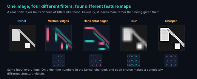
Before any arithmetic, here is what a convolution filter actually does. This output was produced by running the kernel in the middle over the picture on the left.
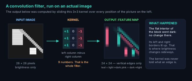
A tiny 3×3 window slid across every position of the image. At each stop it multiplied the nine pixels underneath by nine fixed numbers and added them up, producing one output number.
That is the entire operation. Slide, multiply, add.
Those nine numbers were chosen to compute "left side minus right side". Inside a flat region both sides are equal, so the answer is zero and the output is dark.
At a vertical edge the two sides differ sharply, so the answer is large. The filter found the edges without anyone telling it what an edge is.
These two properties are exactly the two failures on the previous slide, solved.
In a real network nobody chooses those nine numbers. They start random and are learned by exactly the gradient descent from slide 7. The network works out for itself that edge detectors are useful, because edge detectors reduce the loss.
Slide a small weight matrix (the kernel or filter) over the input. At each position take the elementwise product with the patch underneath and sum it to a single number.
Strictly this is cross-correlation. True convolution flips the kernel first. Because the kernel is learned, the flip is irrelevant in practice, and every deep learning framework implements cross-correlation and calls it convolution.
X = 1 2 3 0 1 0 1 2 3 1 1 0 1 2 0 2 1 0 1 3 1 2 1 0 2
W =
1 0 -1
1 0 -1
1 0 -1
# vertical edge
# detector
This kernel computes left column minus right column, summed over three rows. It fires positively on a light-to-dark vertical transition and negatively on dark-to-light.
Top-left 3×3 patch of X:
1 2 3 1 0 -1
0 1 2 ⊙ 1 0 -1
1 0 1 1 0 -1
= (1·1 + 2·0 + 3·-1)
+ (0·1 + 1·0 + 2·-1)
+ (1·1 + 0·0 + 1·-1)
= (1 + 0 - 3) + (0 + 0 - 2) + (1 + 0 - 1)
= -2 + -2 + 0
= -4
Nine dot products, nine outputs, and critically the same nine weights every time. Whatever the kernel has learned to detect, it is detected everywhere at once. That is weight sharing, and it is the single most important structural idea in the architecture.
Notice the output shrank from 5×5 to 3×3. A K×K kernel with no padding loses K-1 pixels in each dimension because the window cannot hang off the edge. Stack ten 3×3 layers and a 32×32 image erodes to 12×12 purely from boundary effects. Padding, two slides on, fixes that.
Nothing changed except the nine numbers in the kernel. Each choice makes a completely different property of the image visible: vertical structure, horizontal structure, smoothness, or fine detail.
A real convolutional layer does not hold one filter. It holds 32, 64, or 256 of them, all applied to the same input, all producing their own output map. The layer then hands that whole stack of maps to the next layer.
| Word | Meaning |
|---|---|
| Kernel / filter | The small grid of learned numbers, typically 3×3 |
| Feature map | The output image one filter produces |
| Channel | One feature map inside the stack. A layer with 64 filters outputs 64 channels. |
A layer with 64 filters of size 3×3
reading a 3-channel colour image:
weights = 3 · 3 · 3 · 64 = 1,728
biases = 64 = 64
───────
1,792
The fully connected layer on slide 11
needed 150,528,000 for the same job.
That is roughly 84,000 times fewer numbers to learn, and the convolutional version is the one that actually works. Fewer parameters is not a compromise here; it is the reason it generalizes.
These four are classic image-processing kernels chosen so the effect is obvious to the eye. A trained network discovers its own, and the early ones do come out looking remarkably like edge and colour detectors — which is a good sign, because it means the network independently rediscovered what human vision researchers found in the 1960s.
with the dilation-adjusted kernel size
| Symbol | Meaning | Typical |
|---|---|---|
I | Input spatial size | 224, 32 |
K | Kernel size | 1, 3, 5, 7 |
S | Stride | 1 or 2 |
P | Zero-padding each side | 0 or (K−1)/2 |
D | Dilation | 1, 2, 4 |
Zero padding is the default but it is a lie about the world: it tells the network there are black pixels outside the frame. reflect and replicate padding avoid that artefact and matter for dense prediction tasks such as segmentation and super-resolution.
| Layer | Computation | Out |
|---|---|---|
| 224, K7, S2, P3 | (224+6−7)/2+1 = 111+1 | 112 |
| 112, maxpool K3, S2, P1 | (112+2−3)/2+1 = 55+1 | 56 |
| 56, K3, S1, P1 | (56+2−3)/1+1 = 55+1 | 56 |
| 56, K3, S2, P1 | (56+2−3)/2+1 = 27+1 | 28 |
| 28, K1, S1, P0 | (28+0−1)/1+1 = 27+1 | 28 |
| 7, K3, S1, P2, D2 | Keff=5; (7+4−5)/1+1 | 7 |
The first two rows are the ResNet stem: 224 → 112 → 56 before a single residual block runs.
Stride 2 halves height and width, which cuts the activation tensor to one quarter the elements and the downstream FLOPs with it. Modern architectures prefer strided convolution over pooling for downsampling because the downsampling itself becomes learnable.
Stacking dilations 1, 2, 4 with 3×3 kernels reaches a 15×15 receptive field in three layers at full resolution: r = 1 + 2 = 3, then 3 + 4 = 7, then 7 + 8 = 15. Semantic segmentation networks (DeepLab) use this to get context without ever downsampling and having to upsample back.
With I = 7, K = 2, S = 2, P = 0 the formula gives ⌊5/2⌋ + 1 = 3, and the last row and column of the input are never read. This is a real and common source of asymmetric behaviour at image borders. Use ceil_mode=True or pad to an even size when it matters.
A conv layer taking C_in channels and producing C_out channels holds C_out filters. Each filter has shape (C_in, K, K) — it spans all input channels at once.
One filter slides over the input and produces one 2-D output map. Stack the C_out maps and you have the output tensor.
The depth dimension of each filter is fully connected; only the spatial dimensions are local and shared. A conv layer is, precisely, a dense layer applied identically to every K×K neighbourhood.
One multiply-accumulate is conventionally counted as 2 FLOPs. Note what is absent from the parameter formula: the spatial size. Note what is present in the MAC formula: the spatial size. Parameters and compute scale completely differently, which is why parameter count is a poor proxy for latency.
Input : 3 × 224 × 224
Filters : 96 of shape (3, 11, 11), stride 4
Output : 96 × 55 × 55
params = (11·11·3 + 1) · 96
= (363 + 1) · 96
= 34,944
MACs = 11·11·3 · 96 · 55 · 55
= 34,848 · 3,025
= 105.4M (≈ 0.21 GFLOPs)
With K = 1 there is no spatial mixing at all, but there is still full mixing across channels. A 1×1, 256→64 conv is a learned linear projection from a 256-dimensional vector to a 64-dimensional vector, applied independently at every pixel.
Parameters: 1·1·256·64 + 64 = 16,448. It is the cheapest way to change channel depth, and it is the workhorse of Inception bottlenecks, ResNet bottleneck blocks, and depthwise separable convolutions. Slide 27 quantifies the saving.
PyTorch defaults to NCHW (batch, channel, height, width); TensorFlow defaults to NHWC. Tensor Cores and most vendor kernels prefer NHWC (channels_last in PyTorch), and switching layout on a ResNet-50 mixed-precision training run is commonly worth 20 to 40 percent throughput for a one-line change. It is the highest-leverage flag most people never set.
Equivariant: shift the input, and the output shifts by the same amount. Convolution is exactly translation-equivariant.
Invariant: shift the input, and the output does not change at all. Convolution is not invariant, and it should not be — for segmentation and detection you need to know where the feature is.
Invariance is manufactured later and deliberately: pooling gives local invariance to small shifts, global average pooling gives full invariance over the image, and data augmentation supplies invariance to the transformations convolution does not handle natively.
| Transformation | Built in? | How it is obtained |
|---|---|---|
| Translation | Yes | Weight sharing |
| Small local shift | Yes | Pooling |
| Rotation | No | Augmentation |
| Scale | No | Image pyramids, FPN, augmentation |
| Illumination | No | Normalization, colour jitter |
| Viewpoint | No | Augmentation, more data |
The honest summary: a CNN is a translation-equivariant model, and every other invariance is bolted on by the training pipeline rather than the architecture.
Compare a dense layer and a conv layer, both mapping a 32×32×3 image to 32×32×64 features:
| Dense | Conv 3×3 | |
|---|---|---|
| Parameters | 201.3M | 1,792 |
| Ratio | 1× | 112,000× fewer |
| Training examples needed | Enormous | Thousands |
dense: 3072 · 65536 = 201,326,592 conv : 3·3·3·64 + 64 = 1,792
Fewer parameters is not the point in itself. The point is that each parameter sees far more training signal: a conv weight receives a gradient contribution from all 1,024 spatial positions of every image, so one image gives it 1,024 effective updates rather than one.
Perfect translation equivariance holds only for stride 1. Any strided layer subsamples, and subsampling without a low-pass filter aliases. Zhang (2019) showed that shifting an ImageNet input by one pixel can flip a ResNet-50 prediction, and that adding a blur before each downsample both fixes much of the instability and improves accuracy. Modern CNNs are approximately, not exactly, shift-equivariant.
The receptive field of a unit is the region of the input image that can influence its value. A layer-1 unit with a 3×3 kernel sees 3×3 pixels. A layer-2 unit sees 3×3 layer-1 units, each of which sees 3×3 pixels, so it sees 5×5.
j is the jump: how many input pixels apart two adjacent units at this layer are. Stride does not grow the receptive field directly — it grows the jump, which then multiplies the growth of every later layer. That compounding is why strided layers are so effective at expanding context.
| Layer | k | s | j | RF |
|---|---|---|---|---|
| input | — | — | 1 | 1 |
| conv1 | 3 | 1 | 1 | 3 |
| conv2 | 3 | 1 | 1 | 5 |
| maxpool | 2 | 2 | 2 | 6 |
| conv3 | 3 | 1 | 2 | 10 |
| conv4 | 3 | 1 | 2 | 14 |
| maxpool | 2 | 2 | 4 | 16 |
| conv5 | 3 | 1 | 4 | 24 |
Eight layers reach 24×24. After the first pool, each 3×3 conv adds (3−1)·2 = 4 pixels rather than 2. After the second pool it adds 8.
Stacked small kernels are strictly better for a fixed receptive field: fewer parameters, fewer FLOPs, and more nonlinearity, which means more expressive power. This is the observation that made 3×3 the near-universal default after VGG in 2014, and it is why 11×11 and 7×7 kernels vanished from everything except the network stem.
The theoretical receptive field is the set of pixels that can influence a unit. Luo et al. (2016) measured the gradient magnitude and found the influence is approximately Gaussian and concentrated in the centre: the effective receptive field grows as O(√L) in depth while the theoretical one grows as O(L).
Practical consequence: a network whose theoretical receptive field just barely covers the object will underperform. Design for a theoretical receptive field two to three times the size of the objects you care about, or add dilation, or add explicit global context such as a pooling pyramid.
Stack two convolutions with nothing between them and the composition is one convolution. Without a nonlinearity, depth buys nothing.
| Activation | Definition | Problem |
|---|---|---|
| Sigmoid | 1/(1+e−x) | Gradient ≤ 0.25; vanishes over depth |
| Tanh | tanh(x) | Saturates at both ends |
| ReLU | max(0, x) | Dead units below zero |
| Leaky ReLU | max(0.01x, x) | Extra hyperparameter |
| GELU / SiLU | x·Φ(x) / x·σ(x) | Costlier to evaluate |
ReLU has gradient exactly 1 for all positive inputs, so the gradient signal does not decay multiplicatively with depth. It is also a comparison and a select, which is far cheaper than an exponential. AlexNet reported reaching a 25 percent training error threshold on CIFAR-10 roughly six times faster with ReLU than with tanh, and that speedup is what made deep CNNs trainable in practice.
If a unit's pre-activation is negative for every input in the dataset, its gradient is zero forever and the unit never recovers. This typically follows a large learning rate driving the bias strongly negative. Symptoms: a large fraction of channels output identically zero, and accuracy plateaus below what the capacity should allow.
Fixes, in order of preference: lower the learning rate, add BatchNorm before the activation, or switch to Leaky ReLU or GELU.
VGG-16 flattens a 512×7×7 map into 25,088 values and feeds three dense layers: 123.6M of its 138M parameters live in that head, roughly 90 percent of the model, doing almost none of the feature work.
fc1: 25088 × 4096 = 102,760,448
fc2: 4096 × 4096 = 16,777,216
fc3: 4096 × 1000 = 4,096,000
─────────────
123,633,664
Global average pooling collapses C×H×W to C by averaging each channel, then a single linear layer maps C→classes. For ResNet-50 that is 2048×1000 = 2.05M parameters instead of 123.6M, and it accepts any input resolution. Introduced in Network-in-Network (2014), adopted by GoogLeNet and everything after.
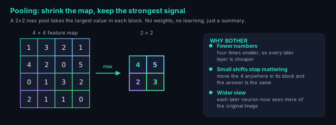
Max pooling discards 75 percent of the activations in a 2×2 window and has no parameters to learn what is worth keeping. Strided convolution downsamples and learns the reduction at the same time, at the cost of parameters and FLOPs. Most post-2015 architectures keep exactly one max pool in the stem and use strided convolution everywhere else. Global average pooling, by contrast, is now universal.
You now have all the parts. This is how they are stacked, and it is the shape of essentially every convolutional network ever built.
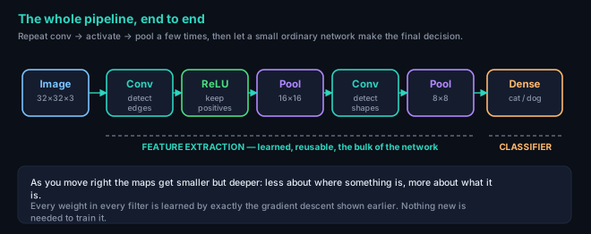
Three operations, repeated a few times:
Then one small fully connected layer turns the final features into a decision. That last layer is exactly the network from Part 1, and it is now doing an easy job because the hard work has already been done.
| Quantity | Direction | Why |
|---|---|---|
| Spatial size | Shrinks: 32 → 16 → 8 | Pooling and striding; exact position matters less as you go deeper |
| Channels | Grows: 3 → 32 → 64 | More kinds of pattern to keep track of |
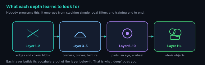
| Meaning | Low to high | From "there is an edge here" to "this is a cat" |
model = nn.Sequential(
nn.Conv2d(3, 32, 3, padding=1), # find edges
nn.ReLU(),
nn.MaxPool2d(2), # 32×32 → 16×16
nn.Conv2d(32, 64, 3, padding=1), # find shapes
nn.ReLU(),
nn.MaxPool2d(2), # 16×16 → 8×8
nn.Flatten(),
nn.Linear(64*8*8, 10), # decide
)
That is a working image classifier. Train it with the identical five-step loop from slide 9 — forward, loss, zero_grad, backward, step. Nothing about training changes.
Everything remaining in this deck is refinement of this picture: how to size the filters and strides precisely, how to keep very deep stacks trainable, what the famous architectures changed, and how the whole thing is made to run quickly. The skeleton above does not change.
For each channel c, compute mean and variance over the batch and both spatial dimensions — that is N·H·W values per channel:
γ and β are learned, giving 2C parameters per layer. They exist so the layer can undo the normalization if that is what minimizes the loss; normalization is offered, not imposed.
Two further buffers, the running mean and running variance, are not learned by gradient descent. They are exponential moving averages updated during training and used in place of batch statistics at inference, so that a single image produces the same output regardless of what it is batched with.
model.train() | model.eval() | |
|---|---|---|
| Statistics used | Current batch | Running averages |
| Running stats | Updated | Frozen |
| Depends on batch peers | Yes | No |
Forgetting model.eval() before validation is the most common bug in this entire field. Symptom: validation accuracy is noisy, far below training accuracy, and changes when the batch size changes. It costs one line and hours of debugging.
BatchNorm estimates statistics from the batch, so the estimate degrades as the batch shrinks. Below roughly 8 to 16 images per device the noise becomes harmful; at batch size 1 the variance is zero and the layer is meaningless. Detection and segmentation, which often run 2 images per GPU because of resolution, hit this constantly. The workarounds are SyncBatchNorm across devices, frozen BatchNorm from a pretrained model, or switching to GroupNorm.
| Variant | Normalizes over | Batch-dependent? | Used in |
|---|---|---|---|
| BatchNorm | N, H, W (per channel) | Yes | Classification CNNs |
| LayerNorm | C, H, W (per sample) | No | Transformers, ConvNeXt |
| InstanceNorm | H, W (per sample, channel) | No | Style transfer |
| GroupNorm | H, W and a group of channels | No | Detection, small batches |
GroupNorm with 32 groups matches BatchNorm accuracy on ImageNet at large batch and clearly beats it below batch size 8, which is why detection frameworks default to it.
The original 2015 paper attributed the benefit to reducing "internal covariate shift". Santurkar et al. (2018) tested that directly by injecting noise after BatchNorm to deliberately increase covariate shift, and training still improved. The explanation that survived scrutiny is that BatchNorm smooths the loss landscape: it bounds the gradient magnitude and makes it more predictable, which permits much larger learning rates.
The practical effects are not in dispute and are large:
Conv → BatchNorm → ReLU # the standard nn.Conv2d(..., bias=False) # bias is redundant: # BN subtracts the mean, # so β absorbs any bias
At inference the BatchNorm affine transform is a per-channel scale and shift, so it can be folded into the preceding convolution weights: the layer disappears entirely and costs nothing. Every deployment toolchain does this automatically, which is why BatchNorm is free in production and only expensive during training.
Augmentation manufactures the invariances convolution does not provide. It is free supervision: no new labels, no new architecture.
| Transform | Invariance taught | Care required |
|---|---|---|
| Random crop + resize | Scale, position | Do not crop the object out |
| Horizontal flip | Left-right symmetry | Wrong for text and digits |
| Colour jitter | Illumination | Wrong if colour is the label |
| Rotation ±15° | Small tilt | 6 and 9 collide at 180° |
| Cutout / random erase | Occlusion | Keep the erased fraction modest |
| Mixup / CutMix | Linear behaviour between classes | Requires soft-label loss |
AlexNet credited random 224×224 crops plus flips from 256×256 images with a large reduction in overfitting; the crop-and-flip pipeline alone multiplies the effective dataset size by more than 2,000.
Random augmentation applied to the validation set makes the metric noisy and pessimistic, and it silently invalidates every comparison you make. Validation should be deterministic: resize, centre crop, normalize. Test-time augmentation is a separate, deliberate technique in which several fixed views are averaged, and it must be applied identically to every model being compared.
| Technique | Mechanism | Typical setting |
|---|---|---|
| Weight decay | Penalize ‖w‖² | 1e−4 (5e−4 for small data) |
| Dropout | Zero units at random | 0.5 in dense heads only |
| DropBlock | Zero contiguous regions | Conv layers, block 7 |
| Label smoothing | Target 0.9 instead of 1.0 | ε = 0.1 |
| Stochastic depth | Skip whole residual blocks | Very deep networks |
| Early stopping | Halt on validation plateau | Patience 10 epochs |
Do not apply weight decay to BatchNorm's γ and β or to bias terms. Shrinking γ toward zero attenuates the signal for no regularization benefit, and excluding those parameters is typically worth a few tenths of a percent of accuracy.
Standard dropout zeroes individual activations independently. In a convolutional feature map neighbouring activations are strongly correlated, so the surviving neighbours carry the dropped information and little is actually removed. Two things replaced it:
ResNet uses no dropout at all in its convolutional trunk; VGG uses 0.5 but only in its dense head.
| Symptom | Diagnosis | Action |
|---|---|---|
| Train ≫ val accuracy | Overfitting | More augmentation, more data, more weight decay |
| Both low, both flat | Underfitting | Bigger model, higher learning rate, train longer |
| Train loss will not fall | Optimization bug | Overfit 10 examples first; if that fails the bug is in the code |
| Val loss rises, val accuracy flat | Overconfidence | Label smoothing; accuracy is still the metric |
| Layer | Output shape | Params | MACs |
|---|---|---|---|
| input | 3 × 32 × 32 | 0 | — |
| conv 3→32, 3×3, p1 | 32 × 32 × 32 | 896 | 0.88M |
| BN + ReLU | 32 × 32 × 32 | 64 | — |
| conv 32→32, 3×3, p1 | 32 × 32 × 32 | 9,248 | 9.44M |
| BN + ReLU | 32 × 32 × 32 | 64 | — |
| maxpool 2×2 | 32 × 16 × 16 | 0 | — |
| conv 32→64, 3×3, p1 | 64 × 16 × 16 | 18,496 | 4.72M |
| conv 64→64, 3×3, p1 | 64 × 16 × 16 | 36,928 | 9.44M |
| maxpool 2×2 | 64 × 8 × 8 | 0 | — |
| conv 64→128, 3×3, p1 | 128 × 8 × 8 | 73,856 | 4.72M |
| global avg pool | 128 | 0 | — |
| linear 128→10 | 10 | 1,290 | 0.001M |
| total | 140,714 | 29.2M |
MACs are per image. Multiply by 2 for FLOPs: roughly 58 MFLOPs per forward pass.
128·4·4 × 512 and more.Stored activations per image (fp32):
conv1 out 32·32·32 = 32,768
conv2 out 32·32·32 = 32,768
pool1 32·16·16 = 8,192
conv3 out 64·16·16 = 16,384
conv4 out 64·16·16 = 16,384
pool2 64·8·8 = 4,096
conv5 out 128·8·8 = 8,192
pool3 128·4·4 = 2,048
─────────
120,832 floats
≈ 0.47 MB per image
batch 128 → ≈ 60 MB of activations
weights → 141K × 4 B = 0.56 MB
Activations exceed weights by more than 100×. Backpropagation must retain every one of them for the backward pass, which is why memory scales with batch size and why gradient checkpointing (recompute instead of store) is the standard remedy when a model will not fit.
def block(cin, cout): return nn.Sequential( nn.Conv2d(cin, cout, 3, padding=1, bias=False), nn.BatchNorm2d(cout), nn.ReLU(inplace=True), ) model = nn.Sequential( block(3, 32), block(32, 32), nn.MaxPool2d(2), block(32, 64), block(64, 64), nn.MaxPool2d(2), block(64, 128), nn.AdaptiveAvgPool2d(1), nn.Flatten(), nn.Linear(128, 10), )
AdaptiveAvgPool2d(1) is global average pooling and works for any input resolution. This model reaches roughly 92 to 93 percent on CIFAR-10 with standard augmentation and a cosine schedule.
Forward pass, dropping batch and channel indices for clarity:
Backpropagation hands us dL/dY, the gradient of the loss with respect to every output element. We need three things: dL/dW, dL/db, and dL/dX to pass upstream.
W[m,n] was used at every output position, so by the multivariable chain rule its gradient sums over all of them:
That expression is itself a cross-correlation: the input correlated with the output gradient. This summation is the mathematical face of weight sharing. A single 3×3 kernel applied to a 56×56 map accumulates 3,136 gradient contributions per image per channel pair, which is exactly why conv weights are so well determined by comparatively little data.
One scalar per output channel: sum the output gradient over batch and both spatial dimensions.
Element X[p,q] contributed to every output whose window covered it. Collecting those terms:
The index signs are flipped relative to the forward pass. Concretely, this is a full convolution of dL/dY with W rotated by 180°, which is precisely the transposed convolution operation. Interior elements receive K² contributions; border elements receive fewer, because fewer windows covered them.
Both backward computations are convolutions. A framework therefore needs one highly optimized primitive, not three, and the backward pass costs roughly twice the forward pass: one convolution for the weight gradient, one for the input gradient.
This 3× rule is the standard estimate for training cost versus inference cost per image, before any optimizer overhead.
| Layer | Backward rule |
|---|---|
| ReLU | Pass gradient where x > 0, zero elsewhere |
| Max pool | Route the full gradient to the argmax; zero to the rest |
| Avg pool | Distribute gradient equally, 1/k² to each input |
| Global avg pool | Broadcast 1/(H·W) across the whole map |
| BatchNorm | Through γ, β, and also through μ and σ², since both depend on x |
Max pooling requires storing the argmax indices from the forward pass, which is why it carries a memory cost despite having no parameters. The BatchNorm backward pass is the subtle one: treating μ and σ² as constants gives a wrong gradient, and it is a classic error in hand-rolled implementations.
torch.autograd.gradcheck(
layer, (x.double().requires_grad_(),), eps=1e-6)
Use float64: float32 rounding swamps the finite-difference estimate and produces failures that look like real bugs. If you ever write a custom convolution kernel, this check is not optional.
| Year | Model | Depth | Params | FLOPs | Top-5 err | The contribution |
|---|---|---|---|---|---|---|
| 1998 | LeNet-5 | 7 | 60K | 0.0005G | MNIST 0.8% | Conv, pool, dense head, trained by backpropagation. Deployed on cheque digits. |
| 2012 | AlexNet | 8 | 60M | 0.7G | 15.3% | ReLU, dropout, heavy augmentation, two GPUs. Beat the runner-up by 10.8 points and ended the hand-crafted-feature era. |
| 2013 | ZFNet | 8 | 60M | — | 11.7% | Smaller stem (7×7 s2 instead of 11×11 s4), found by visualizing what the filters had learned. |
| 2014 | VGG-16 | 16 | 138M | 15.5G | 7.3% | Uniform 3×3 stacks. Proved depth matters and that small kernels beat large ones. 90% of its parameters are in the dense head. |
| 2014 | GoogLeNet | 22 | 6.8M | 1.5G | 6.67% | Inception modules with 1×1 bottlenecks; global average pooling instead of dense layers. 20× fewer parameters than VGG at better accuracy. |
| 2015 | ResNet-50 | 50 | 25.6M | 4.1G | ≈7.1%* | Residual connections plus BatchNorm. Depth stopped being a barrier. |
| 2015 | ResNet-152 | 152 | 60M | 11.6G | 4.49%* | Same idea, 152 layers. The ILSVRC-winning ensemble reached 3.57%, below the ≈5.1% human estimate. |
| 2017 | MobileNetV1 | 28 | 4.2M | 0.57G | ≈10.5% | Depthwise separable convolution throughout. Built for phones, not leaderboards. |
| 2017 | SENet | 154 | 115M | 21G | 2.25% | Squeeze-and-excitation: learn a per-channel gate from global context. Final ILSVRC winner. |
*Reported numbers mix single-model against ensemble and single-crop against multi-crop, so cross-row comparisons are indicative rather than exact. ResNet-50 single-crop top-5 accuracy is approximately 92.9%.
Parameters rose from 60K to 138M and then fell to 6.8M and 25.6M while accuracy kept improving. VGG was the peak of brute force. Everything after it bought accuracy with better structure — bottlenecks, residuals, global pooling — rather than with more weights.
He et al. (2015) trained a plain 20-layer and a plain 56-layer CNN on CIFAR-10. The 56-layer network was worse — on training error, not just test error.
That rules out overfitting entirely. It is also provably not a capacity problem: take the trained 20-layer network, append 36 identity layers, and you have a 56-layer network with at least equal training error. The solution exists in the parameter space. Gradient descent simply could not find it.
The diagnosis: a stack of conv layers finds it hard to represent the identity function, because doing so requires every layer to learn a precisely balanced near-identity mapping.
Rather than asking the block to produce the desired mapping H(x), ask it to produce F(x) = H(x) − x and add x back. Now the identity is the default: drive the weights to zero and the block passes its input through unchanged. A block that is not useful can cheaply become a no-op, so adding depth can no longer hurt.
The gradient view is equally direct. Differentiating the skip path:
The +1 is an unattenuated gradient highway straight to earlier layers. Vanishing gradients require the product of many small factors; the additive identity term prevents that product from ever collapsing.
Plain 3×3 at 256 → 256: 3·3·256·256 = 589,824 Bottleneck 256→64→64→256: 1·1·256·64 = 16,384 3·3·64·64 = 36,864 1·1·64·256 = 16,384 ───────── 69,632 (8.5× fewer)
The 1×1 layers compress to a cheap subspace, do the expensive spatial work there, then expand back. This is what lets ResNet-50 run 50 layers on 4.1 GFLOPs while VGG-16 needs 15.5 GFLOPs for 16.
A standard convolution mixes across space and across channels in one step. Every efficient variant separates those two jobs.
Input 64 × 112 × 112, output 128 × 112 × 112, kernel 3×3.
# Standard convolution MACs = 3·3·64·128 · 112·112 = 73,728 · 12,544 = 924,844,032 # Depthwise: one 3×3 kernel per input channel, # no cross-channel mixing at all MACs = 3·3·64 · 112·112 = 576 · 12,544 = 7,225,344 # Pointwise: 1×1 mixes channels 64 → 128 MACs = 64·128 · 112·112 = 8,192 · 12,544 = 102,760,448 total = 109,985,792 → 8.41× fewer
With K = 3 the 1/K² = 1/9 term dominates once C_out is large, so the saving asymptotes at about 9×. Parameter counts fall by the identical factor: 73,728 becomes 8,768.
Depthwise convolution performs very little arithmetic per byte of memory it touches: each weight is used across one channel only, so there is almost no data reuse to amortize the loads. It is memory-bandwidth-bound, while a standard convolution is compute-bound and sits where GPUs are fastest.
In practice MobileNet's 8.4× FLOP reduction commonly yields 2× to 3× wall-clock speedup on a GPU, and considerably more on a mobile CPU where the compute ceiling is the binding constraint. Measure latency on the target device; never ship a decision made on a FLOP count alone.
| Variant | Params | Mixes space | Mixes channels |
|---|---|---|---|
| Standard K×K | K²·Cin·Cout | Yes | Yes |
| 1×1 (pointwise) | Cin·Cout | No | Yes |
| Depthwise K×K | K²·Cin | Yes | No |
| Grouped, g groups | K²·Cin·Cout/g | Yes | Within group |
| Separable (DW + PW) | K²·Cin + Cin·Cout | Yes | Yes, separately |
Depthwise convolution is grouped convolution with g = C_in. Standard convolution is grouped convolution with g = 1. It is one operator with a single dial.
Split the input channels into g groups and convolve each group only with its own filters. Parameters and FLOPs divide by g exactly. AlexNet used 2 groups purely because the model did not fit on one GTX 580 with 3 GB; the accidental discovery was that it cost almost no accuracy.
ResNeXt made it deliberate, replacing the bottleneck 3×3 with a grouped 3×3 at cardinality 32 and reporting better ImageNet accuracy than ResNet at matched FLOPs and parameters. The cost: groups never exchange information, so ShuffleNet interleaves a channel shuffle between grouped layers to restore cross-group flow.
nn.Conv2d(256, 256, 3, padding=1, groups=32) # 589,824 → 18,432 weights nn.Conv2d(64, 64, 3, padding=1, groups=64) # depthwise: 36,864 → 576 weights
| Technique | Typical gain | Accuracy cost |
|---|---|---|
| INT8 quantization | 4× memory, 2–4× speed | < 1% top-1 |
| FP16 / BF16 | 2× memory, 2–8× on Tensor Cores | None |
| Depthwise separable | 2–3× latency | 1–2% top-1 |
| Structured pruning | 1.5–3× | 0–2%, needs fine-tuning |
| Knowledge distillation | Small model, teacher accuracy | Recovers most of the gap |
| Lower input resolution | Quadratic in FLOPs | Task-dependent, often large |
Reach for mixed precision first. It is one line, it is lossless, and on modern accelerators it is the largest single win available.
Almost every vision task reuses a classification backbone and changes only the head and the loss. This is why ImageNet pretraining transferred so broadly and why backbone improvements propagate to every downstream task at once.
| Family | Approach | Trade-off |
|---|---|---|
| R-CNN (2014) | Region proposals, CNN on each crop | Accurate, ~47s per image |
| Fast R-CNN | One CNN pass, RoI pooling | ~200× faster |
| Faster R-CNN | Learned region proposal network | End to end, ~5 fps |
| YOLO / SSD | Single shot, dense grid prediction | Real time, weaker on small objects |
| RetinaNet | Single shot + focal loss | Fixes class imbalance |
| DETR | Transformer, set prediction | No anchors or NMS, slow to converge |
The recurring problem is class imbalance: a dense detector evaluates roughly 100,000 candidate locations of which a handful contain objects. Focal loss down-weights easy negatives so the rare positives are not drowned out.
Classification collapses space deliberately. Segmentation needs a label per pixel, so the spatial resolution has to be recovered. Transposed convolution is the learnable inverse of a strided convolution:
I=7, S=2, P=1, K=4 O = 6·2 − 2 + 4 = 14 # doubled
Mechanically it is the backward pass of a convolution run forward: each input element is multiplied by the whole kernel and the results are accumulated into an enlarged output.
When K is not divisible by S, output positions receive an uneven number of contributions and a periodic grid pattern appears in the result. The 3×3 stride-2 combination is the classic offender. Two reliable fixes:
K divisible by S, such as 4×4 stride 2.An encoder-decoder alone loses the fine detail during downsampling and cannot invent it back. U-Net concatenates each encoder feature map into the matching decoder stage, so the decoder has both the semantics from the deep path and the boundary precision from the shallow path.
encoder: 572 → 284 → 140 → 68 → 32
│ │ │ │
└──────┴──────┴─────┘ concat
decoder: 32 → 68 → 140 → 284 → 388
It was designed for biomedical images with only 30 annotated training examples, and the skip connections plus aggressive elastic augmentation are what made that possible. The pattern generalized far beyond its original domain, and diffusion models use the same backbone today.
import torch, torch.nn as nn from torchvision import datasets, transforms MEAN, STD = (0.4914, 0.4822, 0.4465), (0.247, 0.243, 0.261) train_tf = transforms.Compose([ transforms.RandomCrop(32, padding=4), transforms.RandomHorizontalFlip(), transforms.ToTensor(), transforms.Normalize(MEAN, STD), ]) # Validation is deterministic. No random transforms. val_tf = transforms.Compose([ transforms.ToTensor(), transforms.Normalize(MEAN, STD), ]) train_ds = datasets.CIFAR10("./data", train=True, download=True, transform=train_tf) val_ds = datasets.CIFAR10("./data", train=False, transform=val_tf) train_dl = torch.utils.data.DataLoader( train_ds, batch_size=128, shuffle=True, num_workers=8, pin_memory=True, drop_last=True) val_dl = torch.utils.data.DataLoader( val_ds, batch_size=256, shuffle=False, num_workers=4)
Normalization constants are the per-channel mean and standard deviation of the training set. Using ImageNet constants on CIFAR is a small but free loss of accuracy, and it is a very common copy-paste error.
device = "cuda" model = build_model().to(device, memory_format=torch.channels_last) opt = torch.optim.SGD( model.parameters(), lr=0.1, momentum=0.9, weight_decay=5e-4, nesterov=True) sched = torch.optim.lr_scheduler.OneCycleLR( opt, max_lr=0.1, epochs=EPOCHS, steps_per_epoch=len(train_dl)) scaler = torch.amp.GradScaler() criterion = nn.CrossEntropyLoss(label_smoothing=0.1) for epoch in range(EPOCHS): model.train() # BN uses batch stats for x, y in train_dl: x = x.to(device, non_blocking=True, memory_format=torch.channels_last) y = y.to(device, non_blocking=True) opt.zero_grad(set_to_none=True) with torch.autocast("cuda", dtype=torch.bfloat16): loss = criterion(model(x), y) scaler.scale(loss).backward() scaler.step(opt) scaler.update() sched.step() # per step, not per epoch model.eval() # BN uses running stats correct = total = 0 with torch.inference_mode(): for x, y in val_dl: x, y = x.to(device), y.to(device) correct += (model(x).argmax(1) == y).sum().item() total += y.numel() print(f"epoch {epoch} val acc {correct/total:.4f}")
model.train() / model.eval() — switches BatchNorm and dropout. Omitting this is the single most common bug in CNN code.zero_grad(set_to_none=True) — gradients accumulate by default; forgetting it silently sums across batches.torch.inference_mode() — no graph is built, so evaluation runs faster and uses far less memory.sched.step() inside the batch loop — OneCycleLR is a per-step schedule; calling it per epoch runs the wrong curve entirely.channels_last plus autocast — commonly 20 to 40 percent throughput for two arguments, with no accuracy change.Early convolutional layers learn edge, colour and texture detectors. Those are properties of natural images in general, not of the 1,000 ImageNet classes. A network trained on ImageNet has already solved the low-level and mid-level vision problem, and your dataset almost certainly does not contain enough examples to solve it again.
Typical outcome on a 2,000-image, 10-class problem: from scratch reaches roughly 60 to 70 percent; fine-tuning a pretrained ResNet-50 reaches roughly 90 to 95 percent, in a small fraction of the training time.
| Your data | Similar to source | Different from source |
|---|---|---|
| Small (< 5K) | Freeze the trunk, train the head only | Freeze early layers, retrain later blocks |
| Large (> 50K) | Fine-tune everything, low learning rate | Fine-tune everything, or train from scratch |
The governing risk with a small dataset is that full fine-tuning at a normal learning rate destroys the pretrained features in the first few hundred steps, before the randomly initialized head has produced a useful gradient signal. Warm up the head first.
A pretrained model expects the normalization statistics it was trained with — for torchvision ImageNet weights, mean (0.485, 0.456, 0.406) and std (0.229, 0.224, 0.225) on RGB in [0,1]. Feeding BGR, or [0,255], or the wrong statistics degrades accuracy in a way that looks like a modelling problem and is not.
from torchvision.models import resnet50, ResNet50_Weights model = resnet50(weights=ResNet50_Weights.IMAGENET1K_V2) for p in model.parameters(): p.requires_grad = False # New head. requires_grad=True by default. model.fc = nn.Linear(model.fc.in_features, NUM_CLASSES) opt = torch.optim.AdamW(model.fc.parameters(), lr=1e-3)
Fast, needs little memory, and hard to get wrong. Also call model.eval() on the frozen trunk during training if you do not want its BatchNorm running statistics to drift toward your small dataset.
# Stage 1: head only, a few epochs, so the head # stops producing garbage gradients. # Stage 2: unfreeze, and give earlier layers a # much smaller learning rate than later ones. for p in model.parameters(): p.requires_grad = True opt = torch.optim.AdamW([ {"params": model.layer1.parameters(), "lr": 1e-5}, {"params": model.layer2.parameters(), "lr": 3e-5}, {"params": model.layer3.parameters(), "lr": 1e-4}, {"params": model.layer4.parameters(), "lr": 3e-4}, {"params": model.fc.parameters(), "lr": 1e-3}, ], weight_decay=1e-4)
Rationale: early layers hold the most general features and need the least change; the head is random and needs the most. A geometric ladder spanning roughly two orders of magnitude is the standard recipe.
The naive implementation is seven nested loops over batch, output channel, input channel, output row, output column, kernel row and kernel column. It has poor locality and cannot use the vendor GEMM kernels that decades of engineering went into. So reshape the problem instead.
Flatten each K×K×C_in patch into a column:
im2col(X) : (C_in·K·K) × (H_out·W_out)
W reshaped: (C_out) × (C_in·K·K)
Y = W_mat @ X_col
: (C_out) × (H_out·W_out)
then reshape Y back to (C_out, H_out, W_out).
The cost is memory. Overlapping windows duplicate every input element roughly K² times, so a 3×3 convolution inflates the input by about 9× in the column buffer. cuDNN chooses per layer between im2col, implicit GEMM which avoids materializing the buffer, FFT, and Winograd.
| Algorithm | Best for | Multiplications |
|---|---|---|
| Direct / GEMM | Anything | Baseline |
| Winograd F(2×2, 3×3) | Small kernels, stride 1 | 36 → 16, a 2.25× reduction |
| FFT | Large kernels (K ≥ 7) | O(N² log N) instead of O(N²K²) |
Winograd trades multiplications for additions and for transform overhead, which is a good trade because multipliers are the scarce resource. It is numerically less stable and is normally restricted to stride 1 with small kernels — that is, exactly the 3×3 layers that dominate modern networks. FFT convolution loses to Winograd at K = 3 because the transform overhead is not amortized.
| Layer type | Bound by | Implication |
|---|---|---|
| 3×3 conv, wide channels | Compute | Runs near peak FLOPs |
| 1×1 conv | Memory bandwidth | Low reuse per byte loaded |
| Depthwise conv | Memory bandwidth | FLOP savings do not fully materialize |
| BatchNorm, ReLU | Memory bandwidth | Fuse into the preceding conv |
| Data loading | Disk and CPU | Frequently the real bottleneck |
Before optimizing the model, profile. A surprising share of "slow training" turns out to be a starved input pipeline: too few dataloader workers, JPEG decoding on the main process, or images being read one at a time from network storage. Watch GPU utilization; if it is not near 100 percent, the model is not the problem.
Total ≈ weights
+ gradients (= weights)
+ optimizer state (2× weights for Adam)
+ activations (batch × per-image)
+ workspace (cuDNN scratch)
ResNet-50, batch 256, fp32:
weights 25.6M × 4 B = 0.10 GB
gradients = 0.10 GB
Adam state = 0.20 GB
activations ≈ 25 MB/img = 6.4 GB ← dominates
Activations dominate by an order of magnitude, and they scale linearly with batch size. The levers, in order: mixed precision (halves activations), gradient checkpointing (recompute rather than store, roughly 30 percent slower for a large memory reduction), then gradient accumulation to simulate a large batch with a small one.
At inference there are no gradients, no optimizer state, and no stored activations beyond the current layer. Fold BatchNorm into the preceding convolution, quantize to INT8, export to a graph compiler (TensorRT, ONNX Runtime, Core ML), and let it fuse conv-BN-ReLU into a single kernel. A ResNet-50 that trains at 4.1 GFLOPs per image routinely serves several times faster than the naive PyTorch eager-mode path suggests.
A CNN has locality, translation equivariance and hierarchy built into the architecture. A Vision Transformer has essentially none of them: it splits the image into patches and applies global self-attention, so it must learn that neighbouring pixels are related.
Strong priors are a loan against data. When training data is limited the prior is correct and free, and the CNN wins. When data is abundant the prior becomes a ceiling, and the model that learns its own structure wins.
| Training data | Winner |
|---|---|
| ImageNet-1k (1.3M) | CNN, clearly |
| ImageNet-21k (14M) | Roughly even |
| JFT-300M | ViT, clearly |
This is the central result of Dosovitskiy et al. (2020): ViT underperforms a comparable ResNet when trained on ImageNet-1k alone, and overtakes it after pretraining on 300M images.
The two families borrowed from each other and largely met in the middle. Swin Transformer reintroduced locality through windowed attention and a hierarchical pyramid. ConvNeXt (2022) took a plain ResNet and applied the transformer-era training recipe and design choices — AdamW, heavy augmentation, LayerNorm, GELU, depthwise 7×7 kernels, fewer activations — and matched Swin at equal FLOPs.
The honest conclusion from ConvNeXt is that a meaningful share of the reported transformer advantage was the training recipe rather than the attention mechanism.
| Situation | Choose | Why |
|---|---|---|
| < 100K labelled images | CNN | Priors substitute for data |
| Edge or mobile deployment | CNN | Mature quantization and kernels |
| Dense prediction, high resolution | CNN or hierarchical ViT | Attention is quadratic in tokens |
| Very large pretraining corpus | ViT | Scales better with data |
| Multimodal with text | ViT | Shares the transformer stack |
| You are unsure | Pretrained CNN | Strongest baseline per unit of effort |
None of these are transformer-free problems. They are consequences of training discriminatively on finite, biased data, and they persist across architectures.
Convolution is not a neural network technique. It is the statement that a useful local operator should be applied uniformly across a signal, and it applies wherever the data has a grid structure with translation symmetry: 1-D over audio and time series, 2-D over images, 3-D over video and volumetric scans. Even in a transformer stack, convolution keeps reappearing in the patch embedding and in hybrid stems, because the underlying claim about signals remains true.
⌊(I + 2P − K_eff)/S⌋ + 1. Learn it once.(K²·C_in + 1)·C_out; MACs multiply that by the output area. They scale differently, so neither predicts the other.O(√depth), not O(depth). Design generously.| # | Check |
|---|---|
| 1 | Overfit 10 examples to near-zero loss. If that fails, the bug is in the code, not the model. |
| 2 | model.eval() before every validation pass. |
| 3 | Normalization statistics match the pretrained weights, or the training set. |
| 4 | No random augmentation on the validation set. |
| 5 | Loss starts near ln(num_classes). For 10 classes that is 2.303. |
| 6 | Labels align with images after shuffling and after augmentation. |
| 7 | Learning rate swept over a log range; it is the highest-impact hyperparameter by a wide margin. |
| 8 | Weight decay excluded from BatchNorm parameters and biases. |
| 9 | GPU utilization near 100 percent, otherwise fix the data pipeline first. |
| 10 | No leakage between train and validation splits, including near-duplicate images. |
nn.Module in depth.