A system design interview guide to typeahead: how to return the most popular suggestions for a prefix in single-digit milliseconds, on every keystroke, by precomputing answers in a trie and rebuilding it offline from query logs.
Student edition · start with the guarantee
Serve ranked prefix completions from a normalized, versioned snapshot without traversing a huge subtree on each keystroke.
Correctness contract: Build and query use the same normalization, locale, filtering, and tie rules. A published snapshot is coherent; stale network responses cannot replace newer input results.
Basic HTTP, databases, and programming are assumed. Specialized terms are explained below. Named products motivate the problem; this is an educational design, not a claim about their current internals. Capacity numbers are illustrative decimal payload estimates, not benchmarks. Add indexes, protocol overhead, replicas, headroom, and failure capacity before provisioning.
Search autocomplete — also called typeahead or search-as-you-type — is the dropdown of suggested completions that appears the moment you start typing into a search box. It looks trivial from the outside, but it has a brutal performance profile: it fires on every keystroke, it must rank suggestions by popularity, and it has to feel instantaneous or it is useless. The trick that makes it work is to split the problem into two independent halves. An online query service answers "given this prefix, what are the top suggestions?" as fast as the network allows, and an offline data-gathering pipeline does all the heavy lifting — counting how often each query is searched and baking those counts into a data structure the query service can read in one hop. This guide walks through both halves, the trie that connects them, and how the whole thing scales.
Each definition includes a concrete example and the condition under which the mechanism is useful. You can read this guide without opening another guide.
Trie and cached prefix top-k
A prefix tree shares character paths between strings. To autocomplete, walk the prefix and return a precomputed list of its highest-ranked completions. A prefix hash map is a simpler alternative for exact-prefix serving.
Example. 'bee', 'beer', and 'best' share 'be'. Cached top-3 for 'be' can return ['best','bee','beer'] without traversing the whole subtree.
Limit. Runtime is O(prefix length+k+output bytes), not literally constant. Normalize consistently, handle absent children, define ranking ties, filter unsafe data, and publish rebuilt snapshots atomically.
Top-k candidate discovery
Frequency estimation and discovering which item IDs to ask about are separate problems. A bounded candidate tracker proposes IDs, then a sketch or exact second pass scores them.
Example. Shard 1 has a=10,x=9; shard 2 has b=10,x=9. Neither local top-1 includes x, but x=18 is the global winner.
Limit. Increasing the local candidate buffer reduces risk but is not a general guarantee. Hash-partitioning each identity to one shard or using a heavy-hitter algorithm with stated bounds changes the analysis.
Cardinality
The number of distinct identities a store must track. A metric series is its metric name plus the full label combination. The product of label-value counts is an upper bound when not every combination occurs.
Example. 100 hosts × 20 routes × 5 status codes can produce up to 10,000 series. Adding a unique request_id can make every request create a new series.
Limit. Hashing every ID to a distinct digest does not reduce cardinality or guarantee anonymity. Use bounded categories, explicit limits, or intentional fixed-bucket aggregation.
Cache-aside and invalidation
A read checks a cache, reads the authoritative store on a miss, then fills the cache. A write commits to the store and invalidates or refreshes the cached value. TTL means time to live, not a freshness proof.
Example. A reader fetches version 1, a writer commits version 2 and invalidates, then the delayed reader caches version 1. DB-first invalidation alone does not prevent this refill race.
Limit. Use invalidation-aware fill leases or version fences for stronger behavior; a TTL only bounds one entry's residence under additional assumptions. Authorization and revocation need an explicit stale-data policy.
DAG scheduling
A directed acyclic graph represents task dependencies. A node becomes runnable only when required predecessors have successfully produced their durable outputs. Acyclic means no dependency cycle, not automatic task termination.
Example. Inspect source video, encode several renditions in parallel, package aligned segments, then conditionally publish a manifest once the required renditions exist.
Limit. Tasks can hang or fail despite an acyclic graph. Use timeouts, bounded retries, attempt identities, cancellation, and atomic completion checks so stale attempts cannot publish bad artifacts.
1. Requirements and Scope
Before touching architecture, pin down exactly what the system must do. Autocomplete has a small functional surface but unusually demanding non-functional requirements, and the design is driven almost entirely by the latter.
For a given prefix, return the k most relevant completions (typically 5 to 10). Not all completions — just the best few that fit in the dropdown.
Ranked by popularity
Suggestions are ordered by how often people actually search them (their historical frequency), so the most likely intent floats to the top.
Extremely fast
The query fires on every keystroke, so a single request must return in a few milliseconds. A common target is a latency budget around 100 ms end to end, including the network round trip.
Prefix match
Suggestions must start with what the user has typed so far. (Fuzzy or mid-word matching is a separate, harder feature usually left out of scope.)
Fresh enough
Rankings should reflect real search trends, but they do not need to be real-time. Trends shift over days and weeks, not seconds.
It is worth being explicit about the load. If a user types a ten-character query, that is up to ten autocomplete requests for a single search. Multiply by every user typing into the box and the read volume dwarfs almost any other endpoint in the product. The flip side is that writes are rare and can be deferred — nobody is editing the suggestion set interactively. That asymmetry (massive reads, lazy writes) is the single most important fact about the design, and it is what licenses the offline-pipeline approach.
A clarifying question worth asking in an interview: do we need to support the full Unicode keyspace, multiple languages, or personalized suggestions? Each of these multiplies the data structure or splits it per-locale. The baseline design below assumes a single language and global (non-personalized) popularity ranking.
Questions to ask before you draw anything:
How many users? Assume 10 million daily active users, 10 searches each per day.
How many suggestions? Top 5 to 10 per prefix [yes].
Spelling mistakes? Fuzzy matching is out of scope for the baseline, discussed later.
Personalized? Global ranking first; personalization as a layer on top.
Filtering? Offensive, dangerous or legally blocked suggestions must never appear [yes].
Intuition
Imagine a librarian who, every Sunday, writes on a sticky note for each set of starting letters ("be", "bee", "bes"...) the five most-asked-for titles. During the week they never search the shelves. They just read the right sticky note. The weekly rewrite is the offline pipeline; the sticky notes are the cached top-k.
2. Back-of-the-Envelope Estimation
Quantity
Working
Result
Daily active users
assumption
10 M
Searches per day
10 M × 10
100 M
Autocomplete requests
100 M × ~20 chars typed
2 B/day
Average QPS
2 B / 86,400 s
≈ 23,000/s
Peak QPS
avg × 2
≈ 46,000/s
Search log growth
100 M × ~100 B
≈ 10 GB/day
Trie nodes
10 M unique queries × 20 chars, ~1/3 kept after prefix sharing
≈ 67 M nodes
Serving trie memory
67 M nodes × ~80 B (children + k=10 pointers)
≈ 5.3 GB
Two conclusions follow. First, a few gigabytes fits in the RAM of one server, so you shard for throughput and headroom more than for size, and you replicate heavily for the 46K QPS. Second, debouncing on the client matters: if it cuts requests per search from 20 to 5, peak QPS drops by 4×.
3. API and Data Model
GET /v1/suggest?q=bes&k=5&locale=en-US
-> 200 { "prefix": "bes", "suggestions": ["best buy", "best restaurants near me", ...] }
   Cache-Control: public, max-age=3600    # same prefix, same answer, for everyone
Data
Where it lives
Shape
Raw search log
Append-only log / object storage
(query, timestamp, locale)
Aggregated counts
Batch output table
(query, frequency) per week, often with a time decay
Trie DB
Durable store (document store or serialized blobs)
Serialized trie or prefix → top-k rows
Serving cache
In-memory on each query server
Trie or prefix hash map, read-only between swaps
Blocklist
Small config store
Terms and patterns never to suggest
4. Two Subsystems
The cleanest way to reason about autocomplete is to separate the read path from the build path completely. They have opposite characteristics — one is latency-critical and runs constantly, the other is throughput-oriented and runs occasionally — so they get different designs, different hardware, and different scaling stories.
The query service (online). A request comes in carrying a prefix; the service looks up the precomputed top-k for that prefix and returns it. This path does almost no computation at request time — that is the whole point. All the expensive ranking work has already been done.
The data-gathering pipeline (offline). This consumes the raw stream of what people searched, aggregates it into per-query frequency counts, builds the data structure the query service reads (a trie), and periodically publishes a fresh copy. It is allowed to be slow because it runs out of the request path.
The contract between the two halves is just the data structure: the pipeline produces it, the query service consumes it. Because the query service only ever reads a finished, immutable snapshot, it never blocks on a build and never sees a half-updated structure. Keeping these subsystems decoupled is what makes the read path simple enough to be fast.
5. The Trie and Cached Top-k
A trie shares character paths. Walk the normalized prefix using a missing-child-safe lookup, then return cached top-k completions. Cost is O(prefix length+k+output bytes); a prefix map avoids traversal but still hashes input and emits output. Do not call it literally constant for unbounded strings.
Build cached lists offline with deterministic ranking ties; compact references need measured memory overhead. Python objects can be much larger than an assumed 80-byte node. Snapshot frequency determines trend freshness. Apply privacy/moderation rules at build and serving if removals need fast effect.
node = root
for char in normalized_prefix:
    node = node.children.get(char)
    if node is None:
        return []
return node.top_k
The downloaded prefix-map model is complete and tested. A production service additionally scopes language/tenant/user policy, authenticates cache keys as needed, publishes versions atomically, and discards stale client responses by request sequence. Fuzzy matching is a different search algorithm, not free from cached exact-prefix lists.
6. The Data-Gathering Pipeline
The trie does not appear from nowhere; it is the output of an offline pipeline that turns raw search activity into ranked suggestions. The pipeline runs on its own schedule, well away from the query service, and publishes finished snapshots for the query service to pick up.
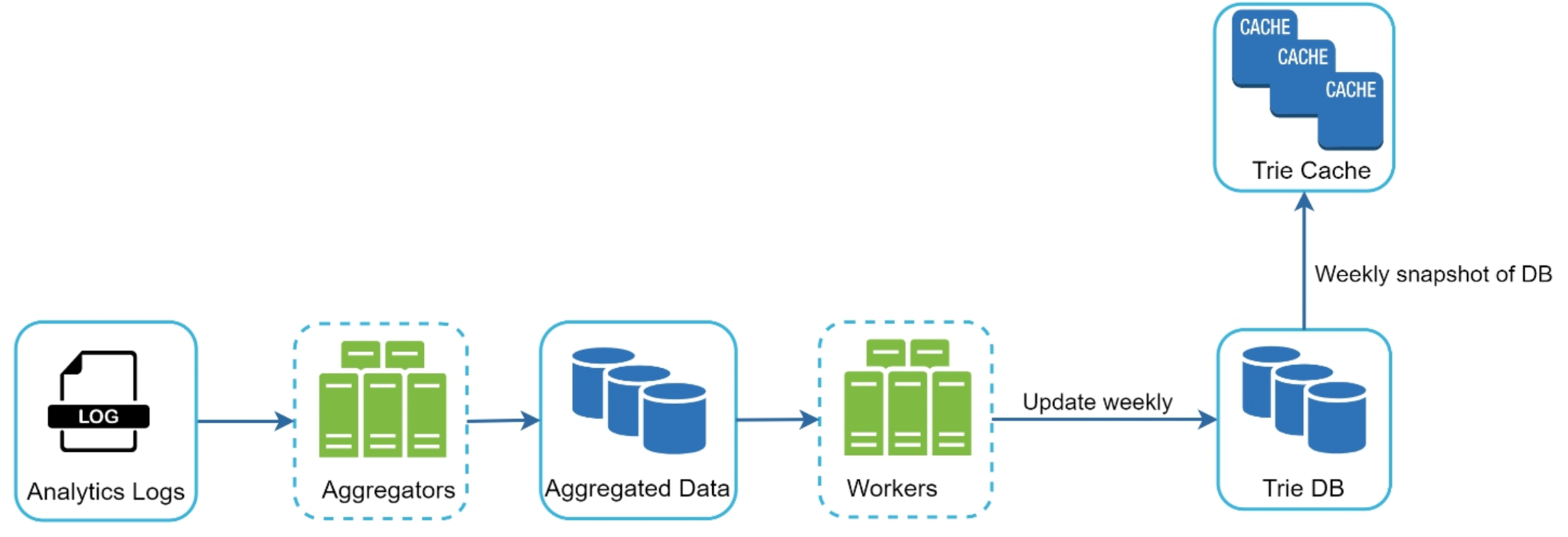
The offline build: Analytics Logs → Aggregators → Aggregated Data → Workers → Trie DB → (weekly snapshot) → Trie Cache, which the query service reads.
The stages are:
Analytics logs. Every search the product serves is logged as a raw event — the query string, and usually a timestamp. This is an append-only firehose; it is the ground truth for what is actually popular.
Aggregators. Jobs read the raw logs and collapse them into frequency counts: how many times each distinct query string was searched over the chosen window. This is a classic group-by-and-count, run as a batch (or windowed) job because the log volume is huge.
Aggregated data. The result is a compact table of (query, frequency) pairs — far smaller than the raw logs, since millions of events collapse into one row per distinct query.
Workers. A set of build workers read the aggregated table and construct the trie. As they insert each (query, frequency) pair they also update the cached top-k lists on the path of nodes leading to that query, so the finished trie has its per-node suggestion lists already populated.
Trie DB. The built trie is persisted to durable storage — the source of truth for the current suggestion data. Holding it in a database (rather than only in memory) means a build can be reproduced, inspected, and reloaded after a restart.
Trie cache (snapshot). Periodically — say weekly — a snapshot of the trie is loaded into the in-memory cache that the query service actually reads from. Publishing a fresh snapshot is how new rankings go live.
# offline build, runs on a schedule (e.g. weekly)
function build_trie(aggregated):           # (query, frequency) rows
  root = new_node()
  for (query, freq) in aggregated:
    node = root
    for ch in query:
      node = node.children.setdefault(ch, new_node())
      offer_to_top_k(node, query, freq)    # keep best k on the path
  persist(root, trie_db)                    # durable source of truth
  publish_snapshot(trie_db, trie_cache)     # swap in for the query service
The defining choice here is that the rebuild is offline and periodic rather than near-real-time, and for autocomplete that is exactly right. Popular-query rankings change slowly: the set of things people search for, and their relative order, drifts over days and weeks, not seconds. A suggestion that was popular yesterday is almost certainly still popular today, so serving rankings that are a few days stale costs essentially nothing in quality. A real-time pipeline that updates the trie on every search would add enormous complexity — concurrent updates to cached top-k lists, contention with the read path, far more infrastructure — to chase freshness the product does not need. Rebuilding periodically lets the build be a clean, batch-shaped, restartable job, and lets the query service treat each published snapshot as an immutable thing it never has to mutate.
If freshness ever does matter — say, surfacing a breaking-news query within minutes — the usual answer is not to abandon the periodic build but to layer a small, fast-updating side index on top of the stable trie, and merge its results at query time. The bulk of suggestions still come from the cheap, slow-moving snapshot.
7. Serving and Scale
The query service exists to do one thing quickly: take a prefix and return its cached top-k. Everything about how it is deployed serves that goal.
Cache the trie in memory. The whole point of the precomputed top-k is defeated if reading a node requires a disk seek. The serving copy of the trie lives entirely in RAM, so a query is a handful of in-memory pointer hops plus reading a short list. The Trie DB is the durable backing store; the Trie cache is the fast serving copy, and the query service reads only the latter.
Shard when the trie outgrows one machine. A trie with cached top-k at every node can grow too large for a single server's memory. The natural way to split it is by prefix — for example, route prefixes starting with a–m to one shard and n–z to another, or shard on the first one or two characters. Because a prefix uniquely determines which shard owns it, the query router can send each request directly to the right shard with no fan-out. The risk is skew: some first letters are far more common than others, so shards are sized by estimated load rather than splitting the alphabet evenly.
Replicate for read throughput. Sharding handles a trie that is too big; replication handles a read volume that is too high. Since the serving trie is read-only between snapshot swaps, replicas are trivial to create — every replica of a shard holds an identical copy, and reads are load-balanced across them. There is no write-consistency problem to worry about because nothing writes to a replica during serving; updates arrive only as a whole new snapshot, which can be rolled out replica by replica.
Technique
Problem it solves
Why it is cheap here
In-memory trie
Per-query latency
Query is pointer hops + a short list read; no disk in the hot path.
Shard by prefix
Trie too large for one machine
Prefix determines the shard, so routing is direct with no fan-out.
Replicate shards
Read volume too high
Read-only snapshots replicate freely; no write-consistency to manage.
8. Client-Side Concerns
A surprising amount of autocomplete's perceived speed and its load profile are controlled in the browser, before a request ever reaches the server. The client is the first line of defense for the latency budget.
Debounce keystrokes. Firing a request on every single keypress is wasteful — a fast typer generates a burst of prefixes most of which are obsolete before a response returns. Debouncing waits for a short pause in typing (say 50–100 ms) before sending a request, so only meaningful prefixes hit the server. This cuts request volume dramatically and avoids showing flickering, out-of-order results.
Cache recent results in the browser. Suggestions for a prefix rarely change between keystrokes, so the client can cache responses locally. When the user deletes a character and retypes, or when one prefix is a continuation of a cached one, the dropdown can be served instantly from the browser with no network call at all.
Respect a tight latency budget. The dropdown has to feel like it is keeping up with the user. With a budget on the order of 100 ms for the full round trip, every layer has to be lean: a debounce window short enough not to feel laggy, an in-memory server lookup, and a small response payload (just k strings). Responses can also carry cache headers so the browser and any CDN edge can reuse them, shaving the round trip on repeated prefixes.
Because typing is sequential, the client can also be smart about ordering: discard any response whose prefix is no longer what is in the box. Without that guard, a slow response for an old prefix can arrive after a newer one and overwrite the correct suggestions.
9. Extensions: Fuzzy, Personal, Safe
Fuzzy matching. Users mistype. One approach walks the trie while allowing a small edit distance (for example 1 typo for short prefixes), exploring a few extra branches. Another indexes common misspellings from query logs as extra keys. Both cost latency, so fuzzy results are usually tried only when exact prefix results are thin.
Personalization. Keep the global trie as is. Separately fetch the user's own recent searches (a small per-user list) and merge them at query time, boosting ones that match the prefix. This keeps the heavy structure shared and cacheable.
Trending queries. A small side index updated every few minutes from a streaming count, merged with the weekly snapshot (see the note above).
Filtering. Apply a blocklist twice: during the build, so bad suggestions never enter the trie, and at serve time, so a newly added term is hidden right away without waiting for the next rebuild.
10. Failure Modes
What breaks
Effect
How to handle it
A query server dies
Lost capacity only.
Stateless read-only replicas behind a load balancer; reload the snapshot on start.
A bad build (bug, poisoned logs)
Wrong or offensive suggestions everywhere.
Validate the new snapshot (size, spot checks, blocklist) before swap; keep the previous snapshot for instant rollback.
Pipeline is late
Suggestions a bit stale.
Keep serving the old snapshot; staleness of a week is acceptable.
Hot prefix (a single letter, a news event)
One shard overloaded.
CDN and browser caching of short prefixes; more replicas for hot shards.
Manipulation (bots searching a phrase)
Spam rises into suggestions.
Count unique users rather than raw searches; rate-limit and filter bot traffic in aggregation.
11. Tradeoffs and Alternatives
Choice
Option A
Option B
Rule of thumb
Structure
Trie with top-k per node
Prefix hash map in a KV store
Hash map is simpler to run; trie saves memory and supports fuzzy walks.
Freshness
Weekly batch rebuild
Streaming updates
Batch for the bulk plus a small streaming side index for trends.
Ranking signal
Raw count
Count with time decay, unique users
Decay and unique-user counts resist stale and spammy terms.
Where to cache
Server memory only
Also CDN and browser
Short prefixes are the same for everyone, so edge caching removes a big share of load.
Worked example: a precomputed prefix map
Counts are best=90, bee=50, beer=40, bet=10; k=3.
Read top to bottom. The table below explains the state and guarantee at each step.
Step
State, calculation, and reasoning
1. Normalize the training strings
Apply the same documented Unicode/case/locale rules used online. Aggregate aliases under that rule and exclude sensitive/unsafe completions before caching.
2. Build prefix be
Collect completions starting with be and rank by descending count, then a deterministic lexical tie rule: best,bee,beer.
3. Look up prefix bee
Return bee,beer from its cached list. An absent prefix returns an empty list, not KeyError.
4. Publish a rebuilt version
Swap an immutable snapshot/manifest atomically. Client request sequence ensures a slow response to 'b' cannot overwrite a newer response to 'bee'.
Check your understanding: Is prefix lookup literally O(1)?
A trie walks O(prefix length); returning suggestions costs O(k+output bytes). Bounded inputs make it fast, not asymptotically constant.
Run a small, testable model
Download concepts.py. It uses only the Python 3.10+ standard library. From the directory where you saved it, run:
python3 concepts.py autocomplete
python3 concepts.py test
The model builds a prefix map, checks deterministic ties and missing prefixes, and prints the worked results.
The program contains deterministic assertions and failure traces. It is a learning model, not a production service: it does not implement network consensus, distributed durability, authentication, or third-party delivery. Read its contracts and try changing an input before extending it.
Top-k by popularity, prefix only, ~100 ms, freshness of days is fine.
5–10
Estimate
~23K QPS (46K peak), 10 GB/day of logs, trie of a few GB.
10–15
API
GET /suggest?q=, cacheable responses.
15–25
High level
Two subsystems: query service with an in-memory trie; offline pipeline from logs to snapshot.
25–38
Deep dive
Top-k cached per node and why; build and swap; sharding by prefix and skew.
38–45
Wrap up
Client debounce and caching, filtering, trends, personalization.
13. Common Mistakes
Mistake 1: traversing the subtree at query time
The prefix s can have millions of completions. Precompute top-k.
Mistake 2: updating the trie on every search
Writes then fight reads for the same structure. Rebuild offline and swap.
Mistake 3: sharding the alphabet evenly
Far more queries start with s than x. Split by measured load.
Mistake 4: forgetting filtering
An offensive suggestion is a real-world incident. Filter at build and at serve time.
Mistake 5: ignoring the client
Without debounce and stale-response guards you pay for extra load and show flickering or wrong suggestions.
14. Summary
Autocomplete is a study in pushing work out of the request path. Almost every design decision trades build-time or memory cost for read-time speed, because the read path is the only thing the user feels.
Concern
Mechanism
How is a query answered fast?
Walk the trie to the prefix node and return its precomputed top-k list — a single node lookup, no subtree traversal.
What is the core data structure?
A trie (prefix tree) where each node caches the top-k most popular completions in its subtree, pre-sorted by frequency.
What is the cost of that cache?
Extra memory: each completion is duplicated across all of its ancestor prefix nodes. Space traded for speed.
A periodic (e.g. weekly) snapshot of the trie is published into the in-memory Trie cache the query service reads.
Why periodic, not real-time?
Popular-query trends drift over days, not seconds, so stale-by-days rankings are fine and avoid huge complexity.
How does it scale?
Trie cached in memory; sharded by prefix when too large; replicated for read throughput since snapshots are read-only.
What does the client do?
Debounce keystrokes, cache recent results, discard stale responses, and stay inside a tight latency budget.
The recurring theme: separate the latency-critical read path from the throughput-oriented build path, precompute every answer the read path could need, and keep the serving structure immutable so it can be cached, sharded, and replicated without coordination. Freshness is bought cheaply with periodic rebuilds because the data underneath changes slowly.
15. Check Yourself
Why store a top-k list at every trie node instead of walking the subtree?
Answer
Short prefixes have huge subtrees. Precomputing makes a query one walk to the node plus reading a short list, trading memory for speed.
10 M users, 10 searches a day, 20 characters each, one request per character. What is the average QPS?
Answer
10 M × 10 × 20 = 2 B requests/day; 2 B / 86,400 ≈ 23,000 QPS.
How would a prefix hash map differ from a trie here?
Answer
Each prefix is a key mapped to its top-k list. Lookup is one get and it fits any KV store, but no nodes are shared, so it uses more memory and cannot be walked for fuzzy matching.
A slow response for "be" arrives after the response for "bes". What should the client do?
Answer
Drop it. Only show a response whose prefix still matches the text in the box.
An offensive phrase starts trending today. Your trie rebuilds weekly. How do you keep it out now?
Answer
Add it to the blocklist, which is also checked at serve time, so it is filtered right away. The next build drops it from the trie.
Why is replicating the serving trie easy?
Answer
It is read-only between snapshot swaps, so every replica is identical and there are no writes to keep in sync.
16. Key Terms
Trie
A prefix tree shares character paths between strings. To autocomplete, walk the prefix and return a precomputed list of its highest-ranked completions. A prefix hash map is a simpler alternative for exact-prefix serving. Example and limits above.
Top-k
Frequency estimation and discovering which item IDs to ask about are separate problems. A bounded candidate tracker proposes IDs, then a sketch or exact second pass scores them. Example and limits above.
Prefix hash map
A key-value map from each prefix to its top-k list.
Debounce
Waiting for a pause in typing before sending a request.
Snapshot swap
Atomically replacing the serving data with a newly built version.
Time decay
Weighting recent searches more than old ones when ranking.
Edit distance
How many single-character edits turn one string into another.
17. Further Reading
Alex Xu, System Design Interview, Volume 1, chapter "Design a Search Autocomplete System."
Edward Fredkin, "Trie Memory," Communications of the ACM, 1960, the origin of the trie.
Bhaskar Mitra and Nick Craswell, "Query Auto-Completion for Rare Prefixes," CIKM 2015, and the survey by Fei Cai and Maarten de Rijke, "A Survey of Query Auto Completion in Information Retrieval," 2016.