Designing a Petabyte-Scale Data Pipeline with Strong SLAs
A system design interview guide to moving petabytes through batch and streaming stages that land correct, complete, and on time — where the hard requirement is not throughput but the freshness and quality guarantee attached to the output.
Student edition · start with the guarantee
Reduce analytical bytes scanned and publish reproducible dataset versions despite task retries and late data.
Correctness contract: Inputs, rule versions, and output manifests identify a reproducible run. Publication is atomic at the table/catalog boundary; quality/completeness policies are explicit.
Basic HTTP, databases, and programming are assumed. Specialized terms are explained below. Named products motivate the problem; this is an educational design, not a claim about their current internals. Capacity numbers are illustrative decimal payload estimates, not benchmarks. Add indexes, protocol overhead, replicas, headroom, and failure capacity before provisioning.
Moving a petabyte is, by now, a solved problem: throw a distributed engine and enough machines at it and the bytes will flow. What makes a petabyte pipeline hard is the promise wrapped around it — that a dataset will be ready by a deadline, complete, correct, and reproducible, every single day, even when an upstream source is late or a schema changes underneath you. That promise is the SLA, and it is what turns a data pipeline from a script into a system. This guide builds such a pipeline: the batch-versus-streaming split (lambda and kappa), ingestion and partitioning, columnar storage with Parquet, a compute engine (Spark or Flink), orchestration and DAGs, and the reliability machinery — data quality gates, schema evolution, lineage, idempotent reprocessing, backfills, and freshness monitoring — that keeps the SLA honest at petabyte scale.
Each definition includes a concrete example and the condition under which the mechanism is useful. You can read this guide without opening another guide.
Partition pruning and predicate pushdown
Pruning excludes storage partitions that cannot match a filter. Column projection reads only requested columns. Predicate pushdown lets file/row-group statistics skip blocks that cannot match; selected blocks still require row filtering.
Example. For a one-day query over a 365-day lake, date pruning can skip 364 days. Min/max time statistics may skip additional row groups only if those statistics are selective.
Limit. Benefits are not universally independent or multiplicative. Row-group sizes, data clustering, skew, metadata, small files, and storage format determine real bytes read.
Inverted indexes and columnar storage
An inverted index maps searchable terms to document postings. A columnar file groups values by column so analytical scans can read only selected fields. They optimize different access patterns.
Example. 'ERROR' → document IDs {2,7}; 'service=api' → {1,2,7}. Intersection returns {2,7}. A monthly count may instead scan only time, service, and status columns.
Limit. Tokenization affects meaning, indexes have storage/write cost, and incomplete shard responses must be marked. Search refresh is visibility, not the same as durable commit.
Offsets and checkpoints
An offset is a position in one log partition. A checkpoint is a recoverable, consistent record of input positions and processing state. On restart, state must correspond exactly to the input that is considered processed.
Example. If a batch increments a total and crashes before saving its offset, replay increments twice. Commit the total, dedup state, and partition position together, or use a compatible transactional/idempotent sink.
Limit. Saving an offset after a write avoids that specific loss window but can still duplicate; framework checkpoints alone do not make arbitrary external effects transactional.
Event time and watermarks
Event time is when the producer says an event happened; processing time is when a consumer handles it. A watermark is the processor's policy-driven estimate of event-time progress, used to emit and eventually clean up window state.
Example. An event for 12:00 arrives at 12:07. A 5-minute allowed-lateness policy may update its window, divert it to correction, or reject it according to the API contract.
Limit. Watermarks are not proof all earlier events arrived. Idle inputs, skew, and unbounded delay require explicit policies; later corrections must propagate to rollups and reports.
DAG scheduling
A directed acyclic graph represents task dependencies. A node becomes runnable only when required predecessors have successfully produced their durable outputs. Acyclic means no dependency cycle, not automatic task termination.
Example. Inspect source video, encode several renditions in parallel, package aligned segments, then conditionally publish a manifest once the required renditions exist.
Limit. Tasks can hang or fail despite an acyclic graph. Use timeouts, bounded retries, attempt identities, cancellation, and atomic completion checks so stale attempts cannot publish bad artifacts.
Transactional outbox
A business transaction writes its state change and an event row to the same database. A relay publishes committed event rows later, retrying until the broker durably accepts them.
Example. An order and its OrderCreated outbox row commit together. A relay crash after publish but before marking sent publishes the same event ID again on restart.
Limit. The relay is at-least-once, not magically exactly-once. Consumers dedup transactionally; preserve per-entity sequence when order matters. CDC is change data capture: reading committed database changes.
1. Requirements & Scope
Intuition
Imagine a library with a million books and one question: how many red books came in on Tuesday? You would not read every book. You go to the Tuesday shelf, look only at covers, and skip boxes labeled “all blue”. That is partition pruning, columnar projection, and min/max stats.
Clarifying questions to ask
Bytes per day, and how long do we keep them?
What freshness do consumers need? Daily tables, or seconds?
Which queries matter most? That picks the partition key.
How much duplication or loss is tolerable? (Usually none.)
How often do schemas change?
What is the compute budget?
At this scale the requirements that matter are the guarantees, not the volume. Anyone can process a petabyte; the design is judged on whether the output can be trusted and whether it arrives on time.
Freshness SLA. Output datasets must be ready by a deadline — daily tables by a certain hour, streaming views within seconds to minutes of the event.
Correctness & completeness. No silent data loss or duplication; the output reflects all and only the intended input.
Quality. Data must pass validation — row counts, ranges, referential checks — before it is published to consumers.
Reproducibility. Re-running a stage on the same input yields the same output (idempotent), so backfills and reprocessing are safe.
Evolvability. Schemas change over time without breaking downstream consumers or historical data.
Cost. At petabyte scale, storage and compute dollars are a first-class constraint, not an afterthought.
2. Back-of-the-Envelope
Numbers show which choices are forced by scale — particularly why columnar storage and partition pruning are not optional.
Quantity
Assumption
Result
Daily volume
~1 PB/day ingested
~12 GB/s sustained average
Event rate
~1 KB events
~10M+ events/sec on the stream
Full-scan cost
read 1 PB at ~10 GB/s aggregate
~28 hours — scanning everything is a non-starter
Partition pruning
query 1 day of a 365 PB year
read 1 PB instead of 365 PB — still ~28 h on its own
Pruning + projection + compression
1 day, 5 of 100 columns, ~5× compressed
1 PB → 50 TB → ~10 TB: ~17 min at 10 GB/s, ~100 s at 100 GB/s
Columnar projection
read 5 of 100 columns
~20× less I/O than row storage
Compression
columnar + zstd on typed data
~3–10× smaller on disk
Worked estimate, step by step
Step
Math
Result
Ingest rate
1 PB ÷ 86,400 s
≈ 11.6 GB/s
Events
11.6 GB/s ÷ 1 KB
≈ 11.6M events/s
Full scan of 1 day
1 PB ÷ 10 GB/s
≈ 28 h
Prune to 1 day of 365
365 PB → 1 PB
1 PB
Project 5 of 100 columns
1 PB × 5%
50 TB
Compressed on disk (~5×)
50 TB ÷ 5
10 TB
Scan time after all three
10 TB ÷ 10 GB/s
≈ 17 min (~100 s at 100 GB/s)
Read the table
Each trick is a multiplier. Pruning, projection and compression together turn 28 hours into minutes. Min/max stats on row groups can cut it further.
The lesson is stark: a full scan of a petabyte takes over a day, so the entire storage design exists to avoid reading data. Partitioning skips irrelevant files, columnar layout skips irrelevant columns, and statistics skip irrelevant row groups. Every query should touch a tiny fraction of the petabyte — that is the whole game.
3. Key Definitions
A few terms recur throughout and are worth fixing precisely.
Term
Meaning
Batch
Processing bounded chunks (e.g. a day) on a schedule — high throughput, higher latency.
Two paths: a fast approximate speed layer plus an accurate batch layer, merged at read.
Kappa
One streaming path; reprocess history by replaying the log — no separate batch code.
Idempotent
Re-running produces the same result — safe to retry and backfill.
Backfill
Reprocessing historical partitions, e.g. after a bug fix or a new column.
Lineage
The recorded map of which inputs produced which outputs.
4. Interfaces & Data Model
A pipeline’s “API” is its table contracts and job definitions.
# table contract (lake / warehouse)
TABLE events (
event_id STRING, user_id BIGINT, event STRING, ts TIMESTAMP, props MAP<STRING,STRING>
) PARTITIONED BY (date DATE, region STRING)
STORED AS PARQUET # row groups ~128 MB, zstd
SORTED BY (user_id) # tight min/max per row group# job contract (orchestrator DAG node)
job daily_user_agg:
inputs: events/date={ds} # waits for partition + quality pass
output: daily_user/date={ds} # atomic overwrite = idempotent
sla: ready_by 06:00 UTC
checks: [ row_count within 20% of 7-day avg, user_id not null ]
Table formats such as Apache Iceberg, Delta Lake or Hudi add atomic commits, snapshots and schema evolution on top of plain Parquet files.
5. Architecture: Lambda & Kappa
Lambda uses batch and speed paths, with a serving policy that avoids double-counting overlapping outputs. Kappa replays a retained log through one processing model. Neither means batch is inherently exact or streaming approximate: exactness depends on accepted inputs, dedup, state/checkpoints, late-data policy, and sink publication.
A single engine/codebase can process bounded and unbounded input, but replay still consumes capacity and requires retained raw data beyond broker expiry. Pin input snapshots and transformation versions so backfills are reproducible. Reconciliation publishes versioned corrections, not a blind overwrite racing the live stream.
6. Storage, Partitioning & Parquet
Since scanning the whole dataset is impossible, storage is designed entirely around reading as little as possible. Two ideas do the heavy lifting: partitioning and columnar format.
Partitioning lays data out in a directory hierarchy by a coarse key — almost always date, often plus region or another high-selectivity dimension. A query filtered to one day then reads only that day’s files (partition pruning), touching a tiny slice of the lake. The art is choosing a partition granularity that prunes well without creating the small-files problem — millions of tiny files that overwhelm the metadata layer and kill throughput. Daily partitions of compacted, appropriately-sized files are the usual sweet spot.
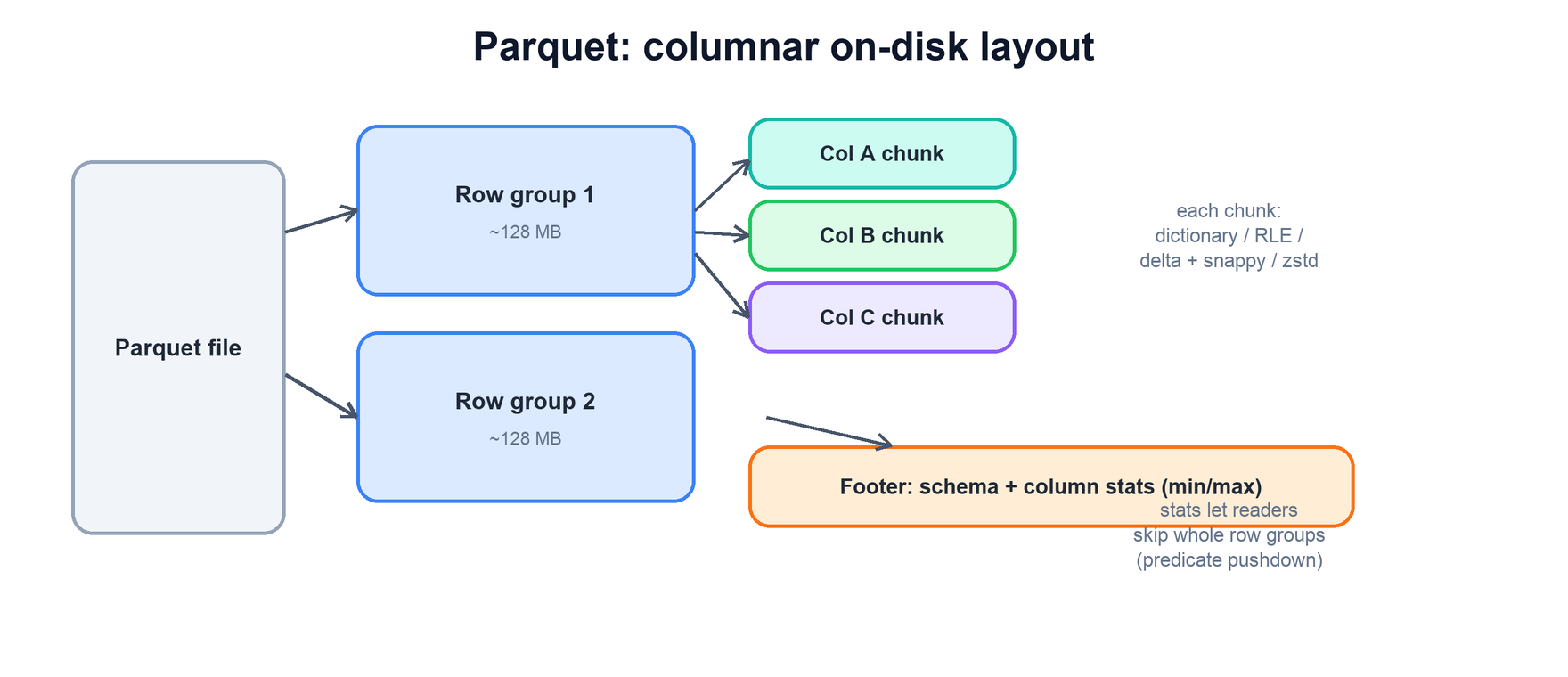
A Parquet file splits into row groups (~128 MB); within each, data is stored column by column as chunks, each encoded and compressed independently. A footer holds the schema and per-column statistics (min/max), letting readers skip whole row groups via predicate pushdown.Every layer of the storage design removes bytes before they are read. The query reads about 10 TB instead of 365 PB.
Parquet is the columnar format that makes analytics affordable. Storing each column contiguously means a query reads only the columns it projects — five of a hundred is roughly twenty times less I/O than a row format. Because a column holds values of one type, encoding is highly effective: dictionary encoding for low-cardinality strings, run-length for repeats, delta for sorted numbers, then a general compressor (snappy for speed, zstd for ratio) on top. And the footer’s per-column min/max statistics enable predicate pushdown: a filter like where ts > X lets the reader skip any row group whose max is below X without decompressing it. Partition pruning, column projection, and row-group skipping compound to turn a petabyte lake into a few gigabytes actually read.
7. Compute: Spark vs Flink
Spark supports batch and Structured Streaming with event-time windows/watermarks; Flink emphasizes managed streaming state and also processes bounded input. Latency and correctness depend on jobs, sources, state, checkpoints, and sinks rather than a universal exact-vs-approximate split.
Exactly-once logical outputs require compatible source replay and transactional/idempotent publication. Checkpoints alone do not atomically publish arbitrary external effects. For a lake, write immutable run files then atomically commit a table/catalog manifest; multi-file object-store rename is usually copy/delete, not an atomic partition swap. Use a reviewed table format/protocol such as Iceberg/Delta/Hudi with its supported writer semantics.
Shuffles co-locate join/group keys and can dominate network cost. Skew needs measured splitting/salting with correct dedup and aggregation semantics. Pin schema/logic/input versions, validate quality, and isolate backfill capacity from freshness-critical jobs.
8. Quality, SLAs & Reprocessing
This layer is what upgrades a pipeline into a system with a promise. Each mechanism protects a specific part of the SLA.
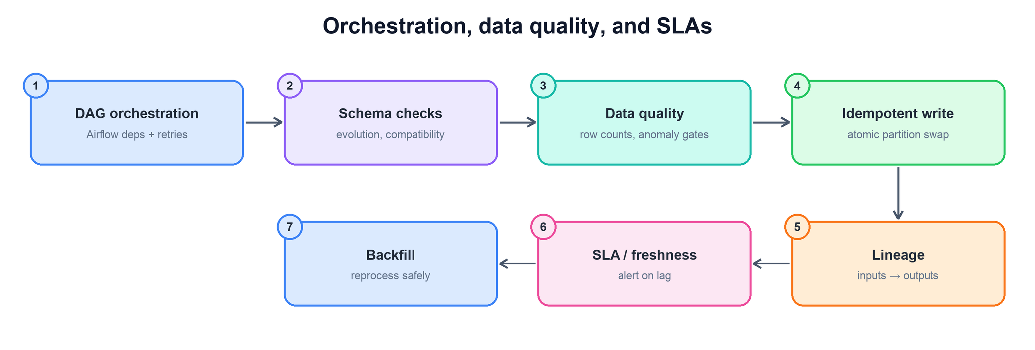
Orchestration sequences the DAG with dependencies and retries; schema and data-quality gates block bad data; idempotent atomic writes make reprocessing safe; lineage tracks inputs to outputs; freshness monitoring watches the SLA; and backfills reprocess history cleanly.
Orchestration & DAGs. A scheduler (Airflow-style) models the pipeline as a directed acyclic graph of tasks with dependencies, retries, and backfill support, so a stage runs only when its inputs are ready and a transient failure retries automatically.
Data quality gates. Before publishing, validate: row-count sanity, null and range checks, referential integrity, distribution anomalies. A failed gate blocks the bad partition rather than poisoning downstream consumers — fail the batch, do not ship garbage.
Schema evolution. Schemas change; a self-describing format plus a schema registry lets you add columns without breaking readers. Enforce backward/forward compatibility rules so old and new data and code interoperate.
Idempotent reprocessing. Writes are idempotent — typically an atomic swap of a whole partition — so re-running a task produces the same result and a retry never duplicates. This is the property that makes everything else safe.
Backfills. When logic changes or a bug is fixed, reprocess historical partitions through the same idempotent jobs. Kappa makes this a log replay; either way, idempotency is the prerequisite.
Lineage. Record which inputs produced which outputs, so you can trace a bad value to its source and know exactly what to reprocess when something is wrong.
SLA / freshness monitoring. Track per-dataset freshness and completeness and alert when a table is late or a partition is missing — the SLA is only real if you are watching it.
Interview tip. When the prompt says “strong SLAs,” anchor your answer on idempotent, atomic partition writes — it is the keystone. It makes retries safe, backfills safe, and exactly-once achievable, and it is what lets you reprocess a petabyte without fear. Pair it with data-quality gates that block bad data before publish and freshness monitoring that alerts on lateness, and you have covered correctness, reproducibility, and timeliness — the three things “SLA” actually means.
9. Bottlenecks & Tradeoffs
The tensions at petabyte scale are about latency versus correctness, and about the cost of every byte read and stored.
Latency vs accuracy. Streaming is fresh but must handle late and out-of-order data; batch is complete but delayed. Lambda buys both at the cost of duplicate logic; kappa keeps one path at the cost of a heavier streaming stack.
Partition granularity. Fine partitions prune better but risk the small-files problem; coarse partitions avoid tiny files but read more per query. Compaction and a daily-ish granularity balance the two.
Shuffle & skew. Joins and aggregations force network shuffles, and skewed keys create stragglers that dominate runtime. Salting hot keys, broadcast joins for small sides, and good partitioning are the mitigations.
Cost vs performance. Better compression (zstd) saves storage but costs CPU; more executors finish faster but cost more. At a petabyte these knobs are budget decisions — optimize the columns read and the data stored first, since I/O dominates.
Schema rigidity vs flexibility. Strict schemas catch errors early but resist change; loose schemas evolve easily but let bad data through. A registry with explicit compatibility rules is the disciplined middle.
10. Failure Modes
Failure
What happens
Defense
Upstream partition late
Downstream runs on partial data
Sensors wait for a completeness marker; alert on lateness
Bad data upstream
Garbage spreads to every consumer
Quality gates block publish; lineage finds what to backfill
Task retried after partial write
Duplicates or half a partition
Write to staging, then atomic swap or table-format commit
Skewed key
One straggler task runs for hours
Salt hot keys; broadcast small side; adaptive query execution
Small-files explosion
Metadata overload; slow listing and reads
Compaction jobs; target 256 MB–1 GB files
Worked example: publishing a retried daily partition
A job computes one day's output from an immutable input snapshot.
Read top to bottom. The table below explains the state and guarantee at each step.
Step
State, calculation, and reasoning
1. Read a pinned input version
Date pruning excludes irrelevant partitions; column projection reads only needed fields. Unequal column widths and already-compressed inputs change sizing.
2. Write run-specific outputs
Workers create immutable files under run_id R1. Retries do not append duplicate visible rows into an existing published partition.
3. Validate before publication
Check schema, row counts, null/range rules, and expected source completeness. Successful batch execution alone does not prove input completeness or business correctness.
4. Atomically commit the manifest
Use a transactional table/catalog compare-and-swap (for example a reviewed lake table format). Ordinary object-store multi-file rename/copy/delete is not atomic partition publication.
Check your understanding: Does batch automatically mean exact and streaming approximate?
No. Both can implement exact effects for a defined input set and lateness policy; either can lose/duplicate or misinterpret inputs without correct state/sink contracts.
Run a small, testable model
Download concepts.py. It uses only the Python 3.10+ standard library. From the directory where you saved it, run:
python3 concepts.py search
python3 concepts.py test
The model checks conservative partition/column pruning; atomic publication is explained as a separate versioned-manifest requirement.
The program contains deterministic assertions and failure traces. It is a learning model, not a production service: it does not implement network consensus, distributed durability, authentication, or third-party delivery. Read its contracts and try changing an input before extending it.
Saying partition pruning alone makes a query fast. One day is still 1 PB here.
Partitioning by a high-cardinality key such as user_id. That makes millions of tiny files.
Appending on retry instead of atomically overwriting a partition.
Publishing data with no quality gate.
Running two codebases (Lambda) without a plan to keep them in sync.
13. Summary
A petabyte pipeline is defined by its promise, not its throughput. The storage layer exists to avoid reading data, the compute layer to process what remains in parallel, and the reliability layer to make the output trustworthy and on time.
Concern
Mechanism
Fresh or accurate?
Lambda runs both a speed and batch layer; kappa uses one streaming path with log replay.
DAG orchestration with retries plus freshness/completeness monitoring and alerting.
The recurring theme: at a petabyte, reading data is the enemy and trust is the product. Lay storage out to read almost nothing, process the remainder in parallel while watching for shuffle and skew, and wrap it all in idempotent writes, quality gates, and freshness alerts — because the deliverable is a dataset that is correct, complete, and on time, every day.
14. Check Yourself
How long does a full scan of 1 PB take at 10 GB/s?Answer
1015 ÷ 1010 = 100,000 s ≈ 28 hours.
A query reads 1 day, 5 of 100 columns, with ~5× compression. How many bytes?Answer
1 PB × 5% = 50 TB, then ÷ 5 ≈ 10 TB. That is about 17 minutes at 10 GB/s.
What is the difference between Lambda and Kappa?Answer
Lambda runs a speed layer and a batch layer with two codebases. Kappa has one streaming path and replays the log to reprocess history.
How do Parquet min/max statistics help?Answer
Each row group stores min and max per column. A filter such as ts > cutoff skips row groups whose range cannot match.
Why must pipeline writes be idempotent?Answer
Retries and backfills then give the same result. An atomic partition overwrite never leaves duplicates.
How does Flink get exactly-once state?Answer
It injects checkpoint barriers into the stream and snapshots operator state asynchronously. Sinks must be transactional or idempotent for end-to-end exactly-once.
15. Key Terms
Partition pruning
Pruning excludes storage partitions that cannot match a filter. Column projection reads only requested columns. Predicate pushdown lets file/row-group statistics skip blocks that cannot match; selected blocks still require row filtering. Example and limits above.
Projection
Pruning excludes storage partitions that cannot match a filter. Column projection reads only requested columns. Predicate pushdown lets file/row-group statistics skip blocks that cannot match; selected blocks still require row filtering. Example and limits above.
Row group
A ~128 MB horizontal slice of a Parquet file.
Predicate pushdown
Pruning excludes storage partitions that cannot match a filter. Column projection reads only requested columns. Predicate pushdown lets file/row-group statistics skip blocks that cannot match; selected blocks still require row filtering. Example and limits above.
Shuffle
Moving data across the network by key.
Skew
One key holding far more data than others.
Watermark
Event time is when the producer says an event happened; processing time is when a consumer handles it. A watermark is the processor's policy-driven estimate of event-time progress, used to emit and eventually clean up window state. Example and limits above.