A system design interview guide to building a log search engine that retains tens of petabytes, indexes them for near-real-time search, and answers a query across a fleet in seconds — the machinery behind systems like Elasticsearch, OpenSearch, and Loki.
Student edition · start with the guarantee
Build a searchable retained log with explicit visibility, durability, query completeness, and authorization boundaries.
Correctness contract: Accepted logs have defined durable copies; refresh visibility is separate from commit. Search responses disclose missing shards and enforce tenant/time filters.
Basic HTTP, databases, and programming are assumed. Specialized terms are explained below. Named products motivate the problem; this is an educational design, not a claim about their current internals. Capacity numbers are illustrative decimal payload estimates, not benchmarks. Add indexes, protocol overhead, replicas, headroom, and failure capacity before provisioning.
Logs are the highest-volume, most detailed telemetry a system produces, and searching them is deceptively hard: you want to type a free-text query and instantly find the handful of relevant lines out of trillions, spanning data from seconds ago to years ago. That requires two ideas working together — an inverted index that maps terms to the documents containing them, so a search never scans everything, and a distributed, tiered architecture that shards the index across many machines and moves aging data down a hot–warm–cold ladder onto cheap object storage. This guide builds that engine: the index model borrowed from Lucene, sharding and time-partitioning, the tiered storage that makes petabytes affordable, and the scatter-gather query path that turns a query string into a plan executed across shards.
Each definition includes a concrete example and the condition under which the mechanism is useful. You can read this guide without opening another guide.
Inverted indexes and columnar storage
An inverted index maps searchable terms to document postings. A columnar file groups values by column so analytical scans can read only selected fields. They optimize different access patterns.
Example. 'ERROR' → document IDs {2,7}; 'service=api' → {1,2,7}. Intersection returns {2,7}. A monthly count may instead scan only time, service, and status columns.
Limit. Tokenization affects meaning, indexes have storage/write cost, and incomplete shard responses must be marked. Search refresh is visibility, not the same as durable commit.
Partition pruning and predicate pushdown
Pruning excludes storage partitions that cannot match a filter. Column projection reads only requested columns. Predicate pushdown lets file/row-group statistics skip blocks that cannot match; selected blocks still require row filtering.
Example. For a one-day query over a 365-day lake, date pruning can skip 364 days. Min/max time statistics may skip additional row groups only if those statistics are selective.
Limit. Benefits are not universally independent or multiplicative. Row-group sizes, data clustering, skew, metadata, small files, and storage format determine real bytes read.
Write-ahead log and fsync
A WAL records updates before data pages are considered committed. Recovery replays it after a crash. fsync (or an equivalent storage contract) requests that buffered bytes reach durable storage rather than only process/OS memory.
Example. A server acknowledges after its WAL commit and required replica writes are durably accepted. A process crash can then reconstruct the committed update.
Limit. Appending to a file alone does not guarantee power-loss durability. Device behavior, filesystem ordering, replicas, corruption, and the declared fault budget still matter.
Offsets and checkpoints
An offset is a position in one log partition. A checkpoint is a recoverable, consistent record of input positions and processing state. On restart, state must correspond exactly to the input that is considered processed.
Example. If a batch increments a total and crashes before saving its offset, replay increments twice. Commit the total, dedup state, and partition position together, or use a compatible transactional/idempotent sink.
Limit. Saving an offset after a write avoids that specific loss window but can still duplicate; framework checkpoints alone do not make arbitrary external effects transactional.
Cardinality
The number of distinct identities a store must track. A metric series is its metric name plus the full label combination. The product of label-value counts is an upper bound when not every combination occurs.
Example. 100 hosts × 20 routes × 5 status codes can produce up to 10,000 series. Adding a unique request_id can make every request create a new series.
Limit. Hashing every ID to a distinct digest does not reduce cardinality or guarantee anonymity. Use bounded categories, explicit limits, or intentional fixed-bucket aggregation.
1. Requirements & Scope
Intuition
Think of the index at the back of a textbook. You do not read every page to find “photosynthesis”. You look it up and jump to pages 42 and 97. An inverted index does that for log lines. Time partitions are like one book per day, so a query about yesterday opens one book.
Clarifying questions to ask
Lines per second, average line size, and retention?
How fresh must search be? Seconds, or is a minute fine?
Full-text on every field, or a few key fields plus grep?
What share of queries are for the last hour versus months ago?
Multi-tenant? Must tenants be isolated?
Do we need aggregations, or only find-the-lines search?
The engine ingests a firehose of log lines and serves search over them. Pin down the requirements.
Functional. Ingest structured and unstructured log lines; full-text and field search with filters (service, level, time range); aggregations (counts, histograms over time); and results ranked or ordered by time.
Near-real-time. A log line should be searchable within seconds of being emitted — incidents happen now, not after a batch job.
Scale. Tens of petabytes retained (exabytes only at the very largest companies), millions of lines per second ingested, queries fanning across thousands of shards.
Query latency. Interactive queries on recent data in well under a second; historical queries over cold data in seconds.
Cost. Retaining petabytes on hot storage is unaffordable; the design must tier aggressively onto cheap object storage while keeping old data searchable.
Custom query language. A DSL that expresses filters, full-text, and aggregations, compiled to a plan executed across shards.
Interview tip: Two ideas carry this whole design — the inverted index (so search is a lookup, not a scan) and time-partitioning + tiering (so most queries touch only recent shards and old data lives on cheap storage). If you anchor on those two, the rest of the design follows naturally.
216 TB/day × ~395 days ÷ ~4× compression ≈ 21 PB. One logical copy: the hot tier adds a replica for a few days only, and object storage handles its own durability.
Index overhead
+10–100% of raw
Full inverted index can equal or exceed raw size — hence index only high-value fields.
Hot tier
~1–2 days on SSD
Most queries hit recent data; keep only days hot, age the rest to warm/cold object storage.
Worked estimate, step by step
Step
Math
Result
Ingest
5M lines/s × 500 B
2.5 GB/s
Per day (raw)
2.5 GB/s × 86,400 s
216 TB/day
Per day (compressed)
216 TB ÷ 4
54 TB/day
Primary shards per day
54 TB ÷ 50 GB target shard
≈ 1,080 shards
Hot tier (2 days, 1 replica)
54 TB × 2 days × 2 copies
≈ 216 TB SSD
Retained 13 months
54 TB × 395 days
≈ 21 PB
Read the table
Only about 1% of the data sits on SSD. The other 99% must live on cheap object storage and still be searchable.
The math drives the architecture directly: index overhead can rival the raw data, so you cannot fully index everything; and retaining PBs is only affordable on object storage, so the design must keep cold data searchable from S3-class storage rather than local disk.
3. The Index Model & Segments
An inverted index maps analyzed terms to postings (document IDs). Analysis/tokenization determines what terms mean. Doc values support sorting/aggregation; numeric/spatial point indexes support range filtering. Immutable segments let readers use snapshots while new segments are added.
Refresh makes recently indexed data searchable, often from filesystem cache. Durability comes from the translog/WAL fsync and replica acknowledgement policy or a durable commit. A Lucene commit persists index state; translog/engine flush reclaims no-longer-needed recovery records under its policy. 'Refresh=searchable, flush=durable' alone is misleading because acknowledged translog-backed writes can be durable before flush.
Replica loss, asynchronous durability mode, or corruption can still lose state outside the declared guarantee. State the configuration, not 'a crash loses nothing' universally. Updates/deletes create version/tombstone bookkeeping; merge reclaims space later.
Field mapping is the data model. service, level and status are keyword fields (exact terms plus doc values). message is analyzed text (tokenized into terms). @timestamp is a date (BKD points for range filters).
5. Sharding & Time-Partitioned Indices
One machine cannot hold petabytes, so the index is partitioned two ways.
Time-partitioned indices
Logs are overwhelmingly queried by recent time, so the primary partitioning is by time: create a new index per day (or hour), e.g. logs-2026-07-06. This is the highest-leverage decision in the design because it makes two things trivial. Queries with a time range touch only the relevant indices and skip the rest entirely (partition pruning). And retention/tiering is a whole-index operation — to expire or move old data you drop or migrate an entire old index, with no per-document deletes.
Shards within an index
Each time index is split into shards — each shard being an independent Lucene index — so ingest and search scale horizontally. A document routes to a shard by hashing a routing key (default the doc id, or a tenant id to co-locate a tenant’s data). Each shard has replicas on other nodes for availability and read throughput. Shard count is a real tradeoff: too few and you cannot parallelize or grow; too many and per-shard overhead and query fan-out costs dominate (the “oversharding” problem).
Partitioning
By
Buys
Time-partitioned index
Event time (per day/hour)
Prune by time; tier/expire whole indices cheaply.
Shard
Hash of routing key
Horizontal ingest & search scale; parallelism.
Replica
Copy of a shard
Availability + read throughput.
6. Ingest & Tiered Storage
Affordability at petabyte scale comes from moving data down a cost/latency ladder as it ages, since query frequency drops sharply with age.
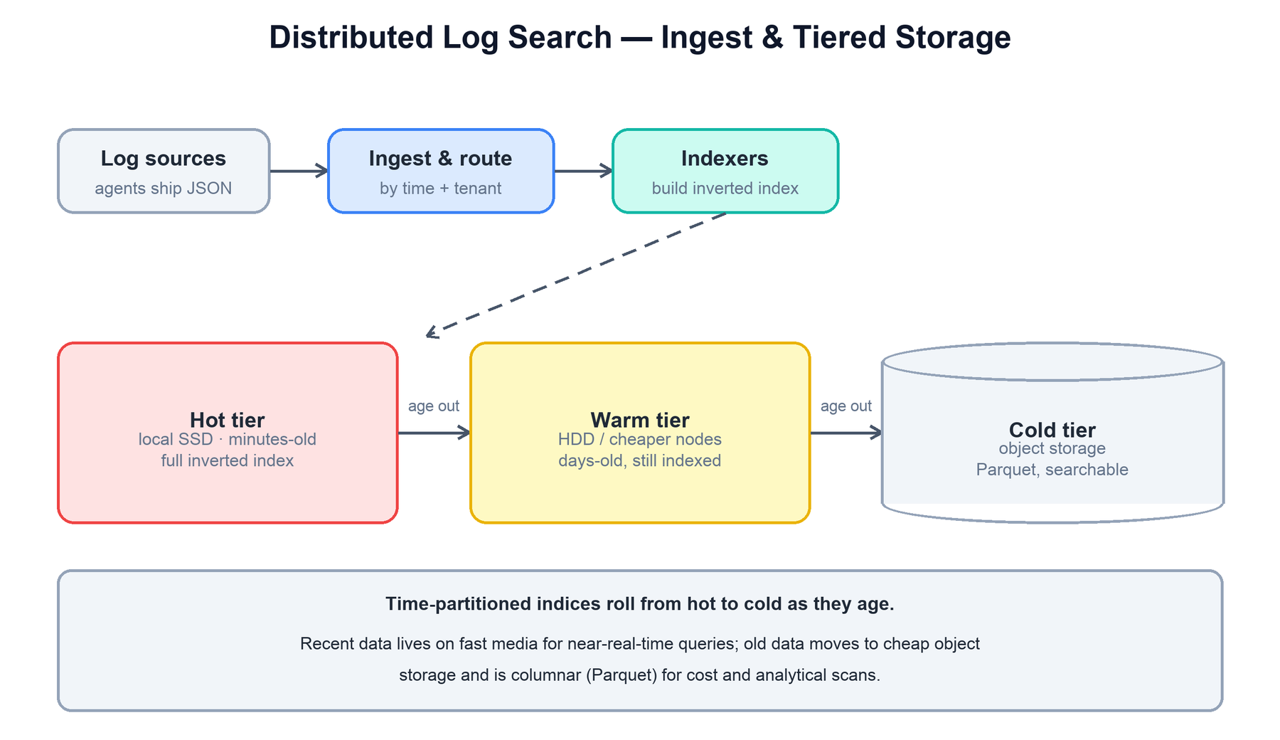
Log sources ship to an ingest layer that routes by time and tenant to indexers, which build inverted-index segments in the hot tier (local SSD, fully indexed, near-real-time). As indices age they roll to a warm tier (cheaper nodes) and then to a cold tier on object storage in columnar (Parquet) form — still searchable, far cheaper.
Hot. Recent indices on local SSD, fully indexed, serving near-real-time ingest and interactive queries. Small, fast, expensive — kept to days.
Warm. Older indices moved to cheaper nodes (more storage, less CPU/RAM), still indexed and searchable but not receiving writes. Read-only and often force-merged into fewer segments for query efficiency.
Cold / frozen. Old indices whose data lives on object storage (S3-class). The node keeps only lightweight metadata and fetches blocks on demand — higher query latency but a fraction of the cost. This searchable-snapshot pattern is what makes retaining petabytes affordable; storage cost decouples from compute.
Data moves down the ladder automatically by index age via a lifecycle policy, and is eventually deleted when it exceeds retention. Because everything is a whole-index operation, tiering is cheap and does not touch individual documents.
7. Query Execution & Scatter-Gather
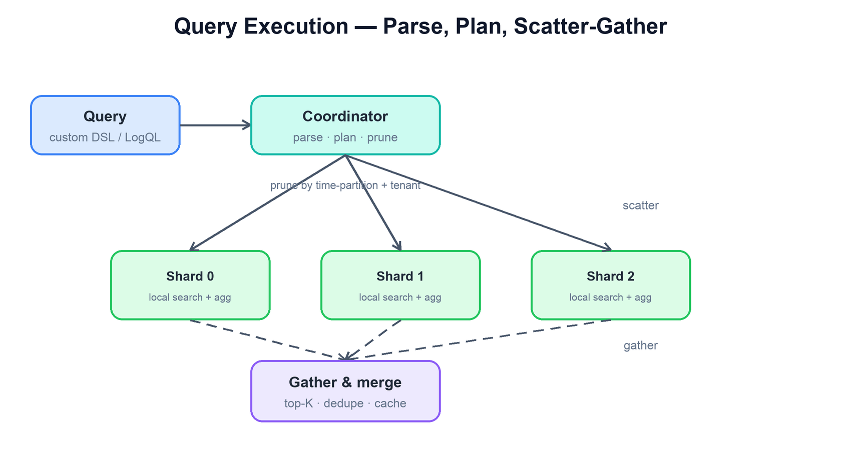
A query is expressed in a DSL and executed in three phases: parse the query string into an AST, plan it (resolve which indices and shards it touches, prune by time and tenant, choose whether to use the inverted index, doc values, or points), and execute it across shards with scatter-gather.
A coordinator parses and plans the query, pruning to only the shards that can hold matching data. It scatters the query to those shards, each of which searches locally and returns partial results; the coordinator gathers, merges (top-K, dedupe), and returns — caching where it can.
The execution model is scatter-gather: a coordinator fans the query to every relevant shard, each shard runs the query against its local segments and returns a partial result (top-K hits, or partial aggregation), and the coordinator merges the partials into the final answer. Two optimizations are essential at scale. Pruning — using the time range to skip whole indices and shards — is what keeps a “last 15 minutes” query from touching a year of data. And caching — of filter results, of frequently hit shards, of aggregation results — absorbs repeated dashboard queries. A two-phase approach (query phase returns just doc ids + scores; fetch phase retrieves the full documents only for the final winners) avoids shipping large documents from shards that will not make the top-K.
function search(dsl, time_range):
  ast     = parse(dsl)                          # -> filters, full-text, aggs
  shards  = plan(ast, time_range)               # prune by time + tenant
  partials = scatter(shards, ast)               # each shard searches locally
  return gather(partials, ast.agg)              # merge top-K / aggregations
8. Columnar Analytics, Caching & Compaction
Three supporting mechanisms round out the engine.
Columnar for analytics. Full-text search wants an inverted index, but analytical queries (“count errors per service per hour over a month”) want to scan a few columns over vast rows — exactly what a columnar format like Parquet excels at. So cold data is stored columnar on object storage: cheap, compressible, and fast to scan for aggregations. Modern systems increasingly split the two — an inverted index for search on hot data, columnar files for analytics on cold data — rather than paying full indexing cost forever.
Caching. Query patterns are heavily repeated (dashboards refresh, alerts re-run), so cache aggressively: OS page cache for hot segments, a query/filter cache for reused predicates, and a results cache for identical dashboard queries. Caching is often the difference between a sub-second and a multi-second dashboard.
Compaction / merging. Because segments are immutable and small ones accumulate, background merging rewrites many small segments into fewer large ones. This bounds the number of segments a query must visit (search cost grows with segment count), and is the only time tombstoned/deleted documents are physically reclaimed. On warm data, an explicit force-merge into a single segment maximizes read efficiency since no more writes are coming.
9. Bottlenecks & Tradeoffs
Index everything vs index selectively. A full inverted index can exceed the raw data in size. Indexing only high-value fields (and storing the rest for scan/columnar) trades some query flexibility for a large cost saving.
Shard count. Too few shards caps parallelism and growth; too many multiplies overhead and query fan-out. Size shards to a target (e.g. tens of GB each) and use time-partitioning to bound their lifetime.
Refresh interval vs cost. Frequent refresh gives lower search latency for new data but creates many small segments and more merge work. Relax it for high-ingest, low-freshness workloads.
Hot storage cost vs query latency. Keeping more data hot is faster but far more expensive; tiering saves money at the cost of higher latency on old data. Tune the ladder to the query-age distribution.
Write vs query contention. Heavy ingest and heavy search compete for the same nodes. Separating write (hot, indexing) from read (warm/cold, query) roles keeps a query storm from stalling ingestion.
10. Failure Modes
Failure
What happens
Defense
Node crash before flush
Recent segments in OS cache are lost
Replay the translog; replicas already hold the data
Ingest spike
Indexers fall behind; search goes stale
Kafka buffer in front of indexers; back-pressure; scale hot nodes
Mapping explosion
Thousands of dynamic fields bloat cluster state
Strict mappings, field limits, store unknown fields unindexed
Route big tenants across more shards; split by tenant + time
Worked example: visibility is not durability
A log is acknowledged, refreshed into searchable segments, and later committed.
Read top to bottom. The table below explains the state and guarantee at each step.
Step
State, calculation, and reasoning
1. Durably accept the log
A translog/WAL and replica policy define survival. OS file-cache visibility alone is not a power-loss guarantee.
2. Refresh for search
Refresh makes new segments visible to readers. It can occur independently of the durable Lucene commit.
3. Search multiple shards
A missing shard yields an explicitly partial response or failed query. Do not silently return incomplete totals as exact.
4. Compact immutable segments
Merge rewrites segments and reclaims deleted data under retention rules. Force-merge consumes resources and is only appropriate for a measured read-only index policy.
Check your understanding: Does refresh prove that acknowledged logs survive power loss?
No. Durability depends on fsynced translog/commit and replica settings, not mere search visibility.
Run a small, testable model
Download concepts.py. It uses only the Python 3.10+ standard library. From the directory where you saved it, run:
python3 concepts.py search
python3 concepts.py test
The model intersects postings and demonstrates date/column pruning against a small exact dataset.
The program contains deterministic assertions and failure traces. It is a learning model, not a production service: it does not implement network consensus, distributed durability, authentication, or third-party delivery. Read its contracts and try changing an input before extending it.
Indexing every field. The index can match the raw data in size.
Keeping all data on SSD. At 21 PB that is not affordable.
Confusing refresh (searchable) with flush (durable).
Oversharding: thousands of tiny shards cost memory and fan-out.
Partitioning only by hash. Time pruning is the biggest win for logs.
13. Summary
A distributed log search engine combines the inverted index (search as lookup, not scan) with time-partitioned, sharded, tiered storage (recent data hot and fully indexed, old data cheap on object storage), executed with scatter-gather across shards.
Concern
Mechanism
How do we search without scanning?
Inverted index: term → postings list; combine terms by set intersection/union.
How are writes made cheap & safe?
Immutable segments, append-only, with a translog for durability; near-real-time via refresh.
How do we scale & prune?
Time-partitioned indices (prune by time) split into hashed shards with replicas.
How do we afford petabytes?
Hot/warm/cold tiers; cold data searchable from object storage (searchable snapshots).
How do we run a query?
Parse → plan (prune) → scatter to shards → gather & merge; cache repeated queries.
How do we serve analytics cheaply?
Columnar (Parquet) for cold data; scan a few columns over many rows.
How do we keep queries fast over time?
Background compaction merges small segments and reclaims deleted space.
The recurring theme: make search a lookup, not a scan, and let time and temperature organize the data. Time-partitioning prunes almost every query down to a slice of the corpus; tiering pushes the vast, rarely-touched majority onto cheap storage; and immutable segments make writes append-only and reads lock-free. The inverted index does the finding; the distributed, tiered architecture makes it affordable at petabyte scale.
14. Check Yourself
How does level:ERROR AND svc:api run without a scan?Answer
Look up both terms in the term dictionary. Fetch their postings lists. Intersect the two sorted lists.
What is the difference between refresh and flush in Elasticsearch?Answer
Refresh writes the buffer as a new searchable segment in the OS cache, with no fsync. Flush is a Lucene commit: it fsyncs segments and trims the translog.
Why partition indices by day?Answer
Time-range queries skip whole days. Retention and tiering move or drop whole indices, with no per-document deletes.
At 54 TB/day compressed and 50 GB shards, how many primary shards per day?Answer
54 TB ÷ 50 GB ≈ 1,080 shards.
Why merge segments?Answer
Each query visits every segment, so fewer segments is faster. Merging is also when deleted documents are really removed.
How can data on S3 stay searchable?Answer
A searchable snapshot keeps small metadata on the node. It fetches and caches the needed blocks from object storage on demand.
15. Key Terms
Inverted index
An inverted index maps searchable terms to document postings. A columnar file groups values by column so analytical scans can read only selected fields. They optimize different access patterns. Example and limits above.