A system design interview guide to predicting when you will run out of hardware — turning utilization telemetry into a demand forecast, a buffer policy, and a procurement order that lands before the wall does.
Student edition · start with the guarantee
Forecast unconstrained demand and purchase enough surviving capacity before lead time runs out.
Correctness contract: Forecasts state uncertainty/calibration, aggregation assumptions, and failure headroom. Procurement uses discrete capacity units and verified lead times.
Basic HTTP, databases, and programming are assumed. Specialized terms are explained below. Named products motivate the problem; this is an educational design, not a claim about their current internals. Capacity numbers are illustrative decimal payload estimates, not benchmarks. Add indexes, protocol overhead, replicas, headroom, and failure capacity before provisioning.
Fleets do not run out of capacity suddenly; they run out predictably, and the failure is almost always organizational rather than technical — nobody ordered the machines in time. Hardware has a long lead time: you cannot conjure a rack the day you need it, so you must see the shortfall coming weeks or months ahead and place the order early. A capacity forecasting system is the machine that makes that foresight routine. It ingests utilization telemetry, models future demand from trend, seasonality, and known growth, translates that demand into hardware and dollars, applies a headroom policy so you never run to the edge, and alerts — with enough runway — when a resource is projected to exhaust. This guide is infra-economics flavored: the output is not a dashboard, it is a purchase order placed at the right time.
Intuition first
Think of filling up a car before a long drive. You know how fast you burn fuel (the trend), that hills burn more (seasonality), and that the next gas station is 100 miles away (the lead time). You refuel when the tank will run low before the next station, not when the light comes on. Capacity forecasting does the same for servers, because new hardware can take months to arrive.
Each definition includes a concrete example and the condition under which the mechanism is useful. You can read this guide without opening another guide.
Forecast percentiles and headroom
A forecast predicts future demand with uncertainty; P50 is a median, not necessarily a mean, and P90 is a quantile under the chosen model. Provision usable surviving capacity above a calibrated demand target.
Example. 6000 units growing 3% per month exceed 7500 usable units after log(7500/6000)/log(1.03)≈7.55 months. A 3.5-month procurement runway means order in about 4.05 months.
Limit. P90 does not mean a 90% chance of never exhausting capacity over the whole horizon. Per-service P90s do not generally add; model correlations, censored demand, lead time, and capacity granularity.
Failure domains and redundant capacity
A failure domain is a set of components vulnerable to one shared event: process, host, rack, zone, or region. Redundancy must separate domains and leave enough surviving capacity to carry peak demand.
Example. Five replicas placed 2/2/1 across three regions leave at least three after any one region fails. A 3/1/1 layout can lose its quorum with the largest region.
Limit. Independent-failure probability formulas are illustrative assumptions. Shared code/config, dependencies, routing, and control planes can fail all replicas together. N+1 machines does not imply tolerance of a whole zone.
SLIs, SLOs, and error budgets
An SLI measures a user-relevant outcome; an SLO sets its target over a window. For a success-ratio SLO, the allowed bad fraction is 1−SLO. An SLA is a contractual commitment that may use different definitions.
Example. 99.9% successful requests over 1 billion requests allows 1 million bad requests. A time-based 30-day availability target instead allows 43.2 unavailable minutes.
Limit. Request and time budgets are not interchangeable under variable traffic or partial failure. SLOs are not universally stricter than SLAs; choose both from their definitions and user needs.
Cardinality
The number of distinct identities a store must track. A metric series is its metric name plus the full label combination. The product of label-value counts is an upper bound when not every combination occurs.
Example. 100 hosts × 20 routes × 5 status codes can produce up to 10,000 series. Adding a unique request_id can make every request create a new series.
Limit. Hashing every ID to a distinct digest does not reduce cardinality or guarantee anonymity. Use bounded categories, explicit limits, or intentional fixed-bucket aggregation.
Backpressure and load shedding
Backpressure tells an upstream producer that the downstream stage cannot accept more work. Buffering delays that signal; shedding deliberately rejects or drops lower-priority work when a bound is reached.
Example. A sink accepts 100 events/s while input is 150/s. A 1000-event queue fills in 20 seconds. The system must then block, reject, or apply its documented drop policy.
Limit. A finite queue cannot absorb an infinite outage. Prioritized messages still need hard quotas, deadlines, and bounded client queues; otherwise an exemption can exhaust the system.
1. Requirements & Scope
The system’s job is to answer one question reliably: for each resource, when will demand exceed supply, and what should we buy to prevent it? Everything else serves that.
Ingest. Collect utilization and growth telemetry across resources — compute, memory, storage, network — per service, region, and hardware type.
Forecast. Project demand forward over the planning horizon, capturing trend, seasonality, and known future events.
Translate. Convert forecasted demand into hardware units and cost, against a headroom/buffer policy.
Alert. Warn when a resource is projected to breach its buffer, with enough lead time to procure before exhaustion.
What-if. Let planners model scenarios — a launch, a migration, a region build-out — and see the capacity impact.
Non-goals. Real-time autoscaling (minutes-scale reaction) is a different system; forecasting operates on the weeks-to-quarters horizon where procurement lives.
Questions to ask first
Which resources: CPU, memory, storage, network, power? At what level: service, cluster, region, fleet?
How long does it take to get new capacity: minutes in a cloud, or months for owned hardware?
What is the cost of running out versus the cost of idle machines?
Are there known events ahead: launches, migrations, holidays, hardware retirements?
Who consumes the forecast: engineers, finance, procurement? What decision does it drive?
2. Back-of-the-Envelope
The numbers here are about horizons and lead times, because those set how far ahead the forecast must see and how early the alert must fire.
Quantity
Assumption
Result
Telemetry cadence
utilization sampled every 1–5 min
plenty of history; downsample to hourly/daily for modeling
Series count
resource × service × region × HW type
tens of thousands of forecastable series
Planning horizon
forecast 2–4 quarters ahead
needs 1–2 years of history to learn seasonality
Procurement lead time
order → racked & serving
weeks to months — the number that matters most
Headroom buffer
N+2 / keep ~20–30% free
survive two failure domains lost (or one during maintenance), plus spikes
Alert runway
fire before exhaustion by
≥ lead time + safety margin
The controlling number is procurement lead time. It defines the alert runway: if hardware takes eight weeks to arrive, a projected-exhaustion alert that fires four weeks out is useless. The whole system exists to convert a slow physical process (buying and racking machines) into a timely one by seeing far enough ahead.
Worked example: when do we order?
A cluster has 10,000 cores and uses 6,000 at peak. Policy keeps 25% free. Demand grows 3% per month, compounding. New hardware takes 3 months to arrive, and we want a 2-week safety margin.
Quantity
Reasoning
Result
Usable capacity
10,000 × (1 − 0.25)
7,500 cores
Annual growth
1.0312
×1.43 per year
Months until usable is exhausted
ln(7,500 / 6,000) ÷ ln(1.03)
7.55 months
Order point
7.55 − 3 lead − 0.5 margin
order within ~4 months
Demand in 12 months
6,000 × 1.0312
8,555 cores
Capacity to cover 12 months
8,555 ÷ 0.75, minus 10,000 owned
buy ~1,406 cores
Growth compounds, so a straight-line guess (“180 cores a month”) gives 8.3 months and orders too late. Always use the compounding formula, and plan on the P90 forecast rather than this single growth rate.
3. Key Definitions
A shared vocabulary keeps the design honest, especially around what “capacity” and “headroom” actually mean.
Term
Meaning
Demand
Forecasted resource need over time — what the workload will consume.
Supply / capacity
Provisioned resource available — what the fleet can serve.
Headroom
Free capacity above current demand — the safety margin.
Buffer policy
The rule for how much headroom to keep (e.g. N+2, or 25% free).
Days-to-exhaustion
Time until forecasted demand crosses the usable-capacity line.
Lead time
Delay from ordering hardware to it serving traffic.
Order point
The moment you must order so hardware lands before the buffer is breached.
The core relationship: order point = exhaustion date − lead time − safety margin. The forecast’s only real purpose is to compute that date early enough to act on it.
4. High-Level Architecture
The system is a pipeline from raw telemetry to a procurement decision, with a planning loop hanging off the middle for what-if analysis.
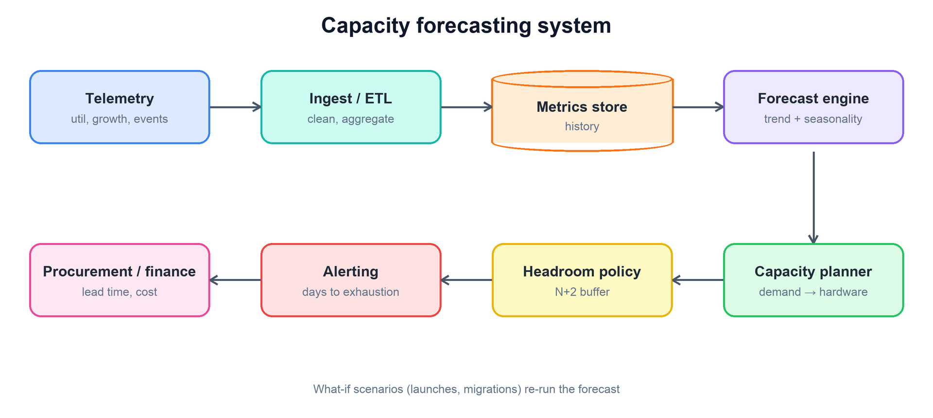
Telemetry flows through ingest/ETL into a metrics store of history; the forecast engine projects demand; the capacity planner translates it to hardware and cost against a headroom policy; alerting watches for projected exhaustion; and results feed procurement and finance. What-if scenarios re-run the forecast.
Telemetry. Utilization, growth, and event signals collected across the fleet, tagged by resource, service, region, and hardware type.
Ingest / ETL. Cleans, normalizes, and downsamples raw samples into the coarser resolution modeling needs, handling gaps and outliers.
Metrics store. A time-series store holding the long history — a year or two — that the models learn from.
Forecast engine. Fits per-series models and projects demand forward with uncertainty bands.
Capacity planner. Converts forecasted demand into hardware units and cost, and compares against supply plus the headroom policy.
Alerting & integration. Fires projected-exhaustion alerts with runway, and feeds the plan to procurement and finance.
5. Modeling Demand
Forecasting demand starts by recognizing that a utilization time series is not random — it is a few structured components plus noise. Decompose it, model each part, and recombine.
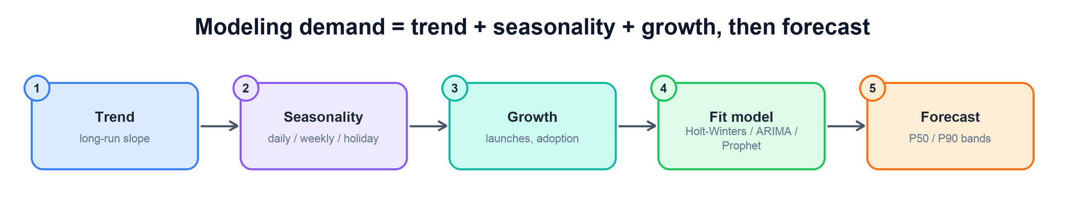
Demand decomposes into a long-run trend, repeating seasonality (daily, weekly, holiday), and known growth (launches, adoption). A model — Holt-Winters, ARIMA, or Prophet — fits these and projects forward with P50/P90 uncertainty bands.
Trend. The long-run slope — steady organic growth or decline.
Seasonality. Repeating cycles: daily peaks, weekly patterns, holiday and end-of-quarter surges. Missing these makes a forecast dangerously optimistic at exactly the wrong time.
Growth events. Known step changes — a product launch, a new region, a migration — that history alone cannot predict and must be injected as regressors.
Residual / noise. What is left after the structured parts — the irreducible uncertainty that sets the width of the confidence band.
Classic model choices: Holt-Winters (exponential smoothing with trend and seasonality) is simple and robust; ARIMA / SARIMA handles autocorrelation and seasonality with more rigor; Prophet is convenient for series with strong seasonality and holiday effects and tolerates gaps. The key output is not a single line but a distribution: forecast at P50 for the expected case and at P90 for planning, because you provision against a pessimistic percentile, not the average. You buy for the bad month, not the typical one.
for series in resources:
  hist   = store.history(series, window="2y")
  parts  = decompose(hist)                # trend + seasonality + residual
  model  = fit(parts, extra=known_events) # inject launches/migrations
  fc     = model.forecast(horizon,
                          quantiles=[0.5, 0.9]) # plan against P90
  publish(series, fc)
Common mistake: forecasting from utilization that hit the ceiling
Measured utilization can never go above 100%. When a service is throttled, queued or shedding load, its graph flattens at the cap, and the model learns that demand has stopped growing. The real demand is hidden. Forecast from request counts or queue depth as well, or mark saturated periods so the model does not trust them.
6. Headroom & Exhaustion
Plan against surviving capacity, not total installed capacity. N+1/N+2 conventionally denotes spare units, not automatically one/two whole failure domains. If one zone holds a third of servers, losing it removes that fraction; include peak load, maintenance, skew, and safe utilization on the remaining fleet.
Find when forecast demand crosses the usable threshold, then subtract procurement, installation, validation, and uncertainty margin. Handle current saturation, zero/negative growth, missing forecasts, and discrete purchase sizes. A 25% free-space buffer is a policy assumption, not proof all failures fit.
P50 is median; P90 is a forecast quantile, not guaranteed 90% survival over an entire horizon. Backtest coverage and model correlations. Do not add per-service percentiles blindly. Forecast uncensored demand from accepted/rejected work and backlog when observed utilization hit a ceiling.
7. What-If & Procurement
The forecast is a baseline; the value multiplies when planners can perturb it and when its output flows straight into the buying process.
What-if scenarios. A planner overlays a hypothetical — “this launch adds 30% load in Q3,” “we migrate service X to a new region,” “we retire this hardware generation” — and the engine re-runs the forecast to show the capacity and cost impact. This turns forecasting from a passive report into a planning tool.
Cost translation. Demand is expressed not just in cores and terabytes but in dollars, using per-unit hardware and running costs, so capacity decisions can be weighed as budget decisions. Infra planning is fundamentally an economics exercise.
Procurement & finance integration. The plan feeds the systems that actually order hardware and hold the budget. An order-point alert becomes a procurement request; the aggregated forecast becomes the quarterly capex ask. The loop closes only when the forecast changes what gets bought.
Interview tip. The signal of a strong answer here is refusing to stop at “fit a time-series model.” Tie the forecast to the physical and financial reality: forecast at a pessimistic percentile (P90, not the mean), alert on the projection against a headroom buffer rather than current usage, and set the alert runway to at least the procurement lead time. The deliverable is a purchase order placed on time, not a pretty chart — say that explicitly.
8. Bottlenecks & Tradeoffs
Forecasting trades the cost of being wrong in one direction against the cost of being wrong in the other, and the design is mostly about choosing which error to prefer.
Over- vs under-provisioning. Provision too much and you burn budget on idle hardware; too little and you hit a wall and take an outage or throttle growth. A bigger buffer and higher percentile favor safety at a cost; the right balance depends on how expensive an outage is versus idle capacity.
Model accuracy vs simplicity. A fancier model may fit better but is harder to trust, explain, and maintain. Simple, robust models (Holt-Winters) that planners understand often beat opaque ones, especially when the output drives real spend.
Horizon vs uncertainty. Forecasts degrade the further out you look, yet lead time forces a long horizon. You manage this by widening bands with distance and re-forecasting continuously as new data arrives, rather than committing once.
Seasonality traps. A model blind to a holiday or quarter-end surge under-forecasts exactly when demand peaks. Capturing seasonality — and injecting known one-off events — is where forecasts most often fail in practice.
Data quality. Garbage telemetry yields garbage forecasts. Gaps, outliers from incidents, and metric changes must be cleaned or the model learns the wrong shape — an outage’s dip should not be read as falling demand.
Worked example: compounding growth meets procurement delay
Current demand is 6000 units, capacity 10,000, reserved headroom 25%, monthly growth 3%.
Read top to bottom. The table below explains the state and guarantee at each step.
Step
State, calculation, and reasoning
1. Compute usable capacity
10,000×0.75=7500 units. Headroom must separately include the defined failed-domain/maintenance scenario.
2. Find threshold crossing
log(7500/6000)/log(1.03)≈7.55 months to usable-capacity exhaustion under this deterministic growth assumption.
3. Subtract lead time
A 3-month lead plus 0.5-month installation margin leaves about 4.05 months until ordering. Already-saturated resources require immediate action, not a negative runway hidden in math.
4. Validate the forecast
Backtest quantile coverage, model correlations, and add known launches. A per-time P90 band is not a 90% no-exhaustion guarantee over the whole year.
Check your understanding: Can P90 forecasts from ten services simply be added?
Not generally. The percentile of a sum depends on dependence; model aggregate demand/correlation. P50 is a median, not always expected demand.
Run a small, testable model
Download concepts.py. It uses only the Python 3.10+ standard library. From the directory where you saved it, run:
python3 concepts.py capacity
python3 concepts.py test
The model calculates runway, uses ceiling for purchased units, and contrasts summed P90s with an independent normal aggregate.
The program contains deterministic assertions and failure traces. It is a learning model, not a production service: it does not implement network consensus, distributed durability, authentication, or third-party delivery. Read its contracts and try changing an input before extending it.
Resources, granularity, lead time, cost of running out vs idle, who uses the output.
5–10
Estimate
Series count, history needed, lead time sets the alert runway.
10–20
Architecture
Telemetry ingest → time-series store → forecasting jobs → plan store → alerts, dashboards, procurement.
20–30
Model
Trend + seasonality + known events; P50 and P90; backtesting to measure error.
30–38
Headroom and order point
Buffer policy, exhaustion date on P90, order point = exhaustion − lead time − margin. Do the worked math.
38–45
Tradeoffs
Over- vs under-provisioning cost, per-series vs aggregate, saturated data, what-if scenarios.
10. Common Mistakes
Mistake
Why it hurts
Do this instead
Planning on the average (P50)
Runs out in half the bad months
Plan on P90 or higher; buffer for model error
Alerting on current usage
By the time it fires, hardware can’t arrive in time
Alert on the forecast crossing usable within the lead time
Linear growth for compounding demand
Orders too late
Fit growth rates; check against the compounding formula
Training on throttled, capped data
Hides real demand
Use request counts; flag saturated periods
Summing per-service P90s
Over-buys shared capacity
Forecast the aggregate; model correlation
Never checking forecast accuracy
Silent drift; nobody trusts the plan
Backtest and track error (for example MAPE) per series
11. Summary
A capacity forecasting system converts slow physical procurement into timely action by seeing demand far enough ahead. Its deliverable is a well-timed order, and every part of the design serves the order point.
Concern
Mechanism
What do we feed the model?
Cleaned, downsampled utilization/growth telemetry with 1–2 years of history.
How do we model demand?
Decompose into trend + seasonality + growth; fit Holt-Winters / ARIMA / Prophet.
What do we forecast against?
A pessimistic percentile (P90) with uncertainty bands — provision for the bad case.
How much slack do we keep?
A headroom buffer (N+2 or ~25% free) subtracted from provisioned capacity.
When do we alert?
When the forecast (not current usage) is projected to breach the buffer within the runway.
How early must the alert be?
At least procurement lead time plus a safety margin — the order point.
How do we plan changes?
What-if scenarios re-run the forecast; output translates to hardware and cost.
How does it drive action?
Integration with procurement and finance turns alerts into orders and capex plans.
The recurring theme: forecasting is an economics problem with a deadline. See demand far enough ahead, plan against a pessimistic percentile with a headroom buffer, and fire the alert a full lead time before the wall — because the only forecast that matters is the one that gets the hardware ordered in time.
12. Check Yourself
Hardware takes 10 weeks to arrive and your alert fires 6 weeks before projected exhaustion. What is wrong?
AnswerThe runway is shorter than the lead time. The alert must fire at least 10 weeks plus a margin before exhaustion, or the capacity arrives after you run out.
Usage is 4,000 units, usable capacity is 5,000, and demand grows 2% per month. About how many months until exhaustion?
Answerln(5,000 / 4,000) ÷ ln(1.02) ≈ 11.3 months.
Why plan against P90 instead of P50?
AnswerP50 is exceeded half the time. Running out is usually far more costly than a little idle capacity, so you plan for the pessimistic but plausible case.
A service’s CPU graph has sat flat at 100% for two weeks. What does that tell the forecaster?
AnswerDemand is being capped, so true demand is unknown and probably higher. Those points should not be trusted as demand; use request or queue metrics instead.
What does N+2 protect you against?
AnswerLosing two failure domains at peak, or more commonly one planned for maintenance plus one unplanned failure at the same time.
How do you know your forecasting model is any good?
AnswerBacktest it: train on data up to a past date, forecast the next months, and compare with what really happened. Track an error metric and check how often reality falls outside the P90 band.
13. Key Terms
Lead time
Time from ordering capacity to it serving traffic.
Headroom
Capacity kept free on purpose.
Usable capacity
Provisioned capacity minus the buffer.
Exhaustion date
When forecast demand crosses usable capacity.
Order point
Exhaustion date minus lead time minus margin.
Trend
Long-run direction of demand.
Seasonality
Cycles that repeat daily, weekly or yearly.
P50 / P90
Values that demand stays under 50% / 90% of the time.
Backtesting
Testing a model on past data it has not seen.
N+1 / N+2
Enough capacity to lose one / two failure domains.