← CatZep/Engineering Guides/System Design/Counting & Analytics

Trending Topics and Top-K

A system design interview guide to finding the most frequent items in a massive stream — trending hashtags, top products, hottest search terms — when the universe of items is too large to count exactly and "trending" means recency, not all-time totals.

"Show me the top ten trending hashtags" is a question every social product answers, and it hides a genuinely hard counting problem. The stream of items is unbounded and the set of distinct items — hashtags, product ids, search queries — runs into the millions or more, most of them rare. Keeping an exact counter for every item so you can sort and take the top k means a hash map the size of the entire item universe, updated on every event. The way out is to give up exactness for the long tail you do not care about while staying accurate for the heavy hitters you do, using a probabilistic frequency sketch paired with a small heap. This guide builds that design up, then extends it to the recency that makes a count "trending" and to merging results across shards.

Concepts to understand first

Each definition includes a concrete example and the condition under which the mechanism is useful. You can read this guide without opening another guide.

1. The Top-K Problem

The Top-K problem is: given a stream of items where the same item appears many times, report the k items with the highest frequency. It sounds like a sorting problem, but the scale changes its character — you cannot afford to keep an exact, sorted tally of a stream that never ends over a universe of items that is enormous and mostly irrelevant.

The applications are the recommendation and discovery surfaces of almost any product:

• Trending hashtags or topics — the tags appearing far more than usual right now, surfaced on a discovery page.
• Top products — the most-viewed or most-purchased items, for a "popular now" rail or merchandising.
• Hottest search queries — the queries spiking in volume, for autosuggest and editorial surfacing.

What makes this its own design topic, distinct from plain distinct-counting, is the shape of the data. Item frequencies follow a heavy-tailed distribution: a handful of items are wildly popular and the overwhelming majority appear only a few times. You only ever care about the head of that distribution — the top k — yet an exact approach is forced to spend memory tracking the entire tail just in case. The whole game is to be accurate about the heavy hitters while refusing to pay for the millions of items that will never come close to the top.

2. Requirements and Clarifying Questions

• Top what, and how many? Search queries, hashtags, products? (Assume search queries, k = 100.)
• Over what window? All time, last hour, last day? Sliding or fixed? (Assume last hour and last day, refreshed every minute.)
• Exact or approximate? Does the 100th item have to be exactly right? (Assume approximate; order near the top matters most.)
• Popular or trending? Highest count, or biggest rise compared with usual? (Start with popular, then extend.)
• Global or per region? (Assume global plus per country.)

3. Back-of-the-Envelope Estimation

Assume 500 million searches a day, a 3× peak, 100 million distinct queries a day, and about 88 bytes per exact map entry (a ~50-byte string, an 8-byte count, and hash-table overhead).

An hourly top-100 query is typically searched tens of thousands of times, so a worst-case overcount of about 208 barely moves the ranking. The sketch is about 1,600× smaller than the exact map, and it does not grow on a day with twice as many distinct queries.

4. Why Exact Top-K Is Expensive

The exact solution is a hash map from item to count, incremented on every event, with the top k read off by sorting (or maintaining a heap). It is correct, and at small scale it is fine. The cost problem is the size of the map, and it is driven by the long tail rather than the heavy hitters.

Because the map needs an entry for every distinct item that has ever appeared, its memory scales with the size of the item universe, not with k. In a heavy-tailed stream the universe is dominated by rare items — millions of hashtags used once or twice — and you are paying to store a counter for every single one of them, even though none will ever be in the top ten. You are spending almost all of your memory on items the answer will never mention.

At stream scale this map becomes too large to hold in memory on one machine, which forces it into a distributed store and turns every increment into a network operation against hot keys. The exact approach is not wrong; it simply ties memory to the wrong quantity — the breadth of the tail — when the question only concerns the head.

The escape, as with distinct counting, is a tolerance the consumer already has: a trending list does not need exact counts, only the right items in roughly the right order. If item frequencies are estimated with a small, bounded error, the ranking of the heavy hitters is preserved, and the rare items can be allowed to collide and share space because their exact counts never mattered. That tolerance is what the Count-Min Sketch exploits.

5. Count-Min Sketch

A Count-Min Sketch (CMS) is a compact, fixed-size structure that estimates how many times each item has been seen, using far less memory than an exact map by deliberately letting different items share counters. It is the frequency analogue of the bit tricks behind cardinality sketches: trade a little accuracy for a memory footprint that does not grow with the item universe.

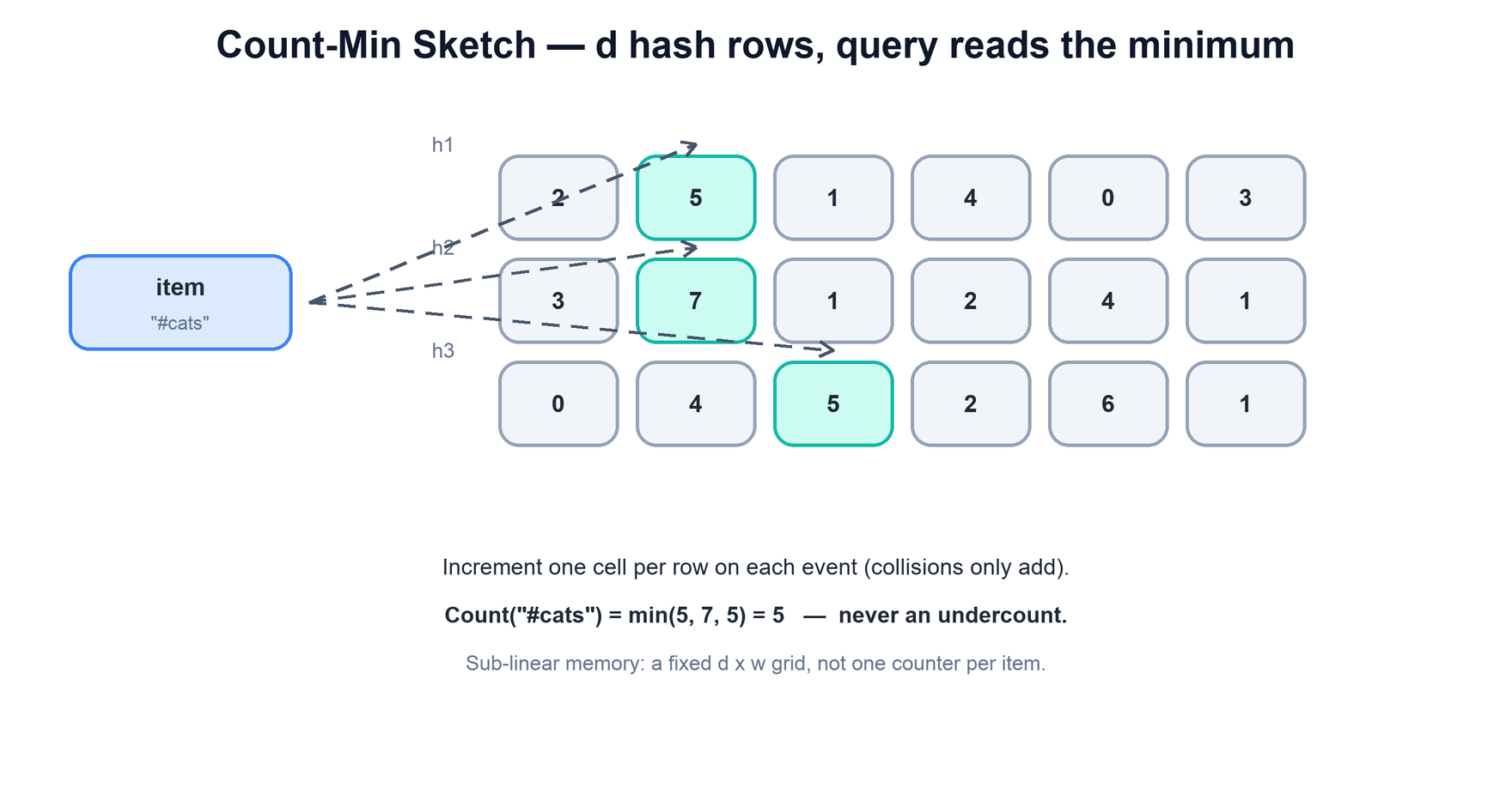
Structurally a CMS is a two-dimensional array of counters: d rows and w columns, with one independent hash function per row. To record an item, you hash it once per row to pick one column in that row and increment all d of those counters. Different items may hash to the same column in some row — a collision — and when they do they share that counter, which is the source of both the memory savings and the error.

The clever part is the query. To estimate an item's count you look at its d chosen counters — one per row — and take the minimum. Every one of those counters includes the item's true count plus whatever other items happened to collide with it in that cell, so each counter is an overestimate. The minimum is the least-contaminated of them, the cell where the fewest other items landed. This gives a one-sided guarantee that is exactly what Top-K needs: the estimate is never below the true count, and only ever an overestimate, with the overshoot bounded by the sketch's dimensions.

# increment: one cell per row, all d rows
function cms_add(cms, item, count=1):
  for r in range(d):
    c = hash[r](item) % w          # this row's column for the item
    cms[r][c] += count             # shared cell — collisions just add

# query: minimum over the d cells is the least-contaminated estimate
function cms_estimate(cms, item):
  return min(cms[r][hash[r](item) % w] for r in range(d))   # never an undercount

The memory win is that the grid is a fixed d × w size chosen for the accuracy you want, completely independent of how many distinct items the stream contains. Adding a millionth rare hashtag costs nothing — it just collides into existing cells — whereas the exact map would allocate a new entry. The structure is sub-linear in the item universe by construction.

6. Pairing CMS with a Heap

A CMS estimates the frequency of any item you ask about, but on its own it cannot tell you which items are the top k — it has thrown away the identities. To produce the actual list you pair the sketch with a small min-heap of size k that remembers the current leading items and their estimated counts.

The heap holds at most k entries and is ordered so that its root is the smallest estimate among the current leaders — the weakest member of the top k, and therefore the one most easily displaced. This is the standard structure for "keep the largest k things seen so far," and keeping it at exactly size k means it costs a tiny, fixed amount of memory regardless of stream length or item universe.

The two structures divide the labour cleanly. The CMS answers "how often has this item been seen?" in fixed memory; the heap answers "is that frequent enough to be in the current top k, and if so who does it bump?" Neither could do the job alone: the sketch lacks identities, and a heap over raw counts would need the exact per-item tallies the sketch is there to avoid.

7. API and Data Model

# write: the search service emits one event per query (async, via Kafka)
{ "item": "world cup final", "ts": "2026-09-25T14:03:07Z", "country": "BR" }

# read: precomputed, served from cache
GET /v1/top?window=1h&country=BR&k=10
  → { "as_of": "2026-09-25T14:03:00Z", "approximate": true,
      "items": [ { "item": "world cup final", "count": 184220 }, … ] }

8. The Streaming Algorithm

Each insertion costs O(d) CMS updates plus the candidate tracker's cost. An indexed heap can update a known candidate in O(log k); scanning a Python list of names and heapifying costs O(k). For fixed small k that may be a reasonable demo, but it is not the same algorithmic bound.

CMS collisions can increase a candidate's estimated count when another item is inserted. Heap scores refreshed only on that candidate's own arrivals can therefore be stale. Re-score the retained candidates before reporting a snapshot and document the tracker as a heuristic unless it has a proved discovery bound. A CMS does not itself retain names or make top-k membership exact.

At a window boundary, sum compatible live-bucket sketches and rebuild scores from a sufficient candidate set. Bucket approximation cannot answer arbitrary partial-bucket windows exactly. Subtracting a whole saved bucket from a matching running grid can be safe algebraically; arbitrary negative updates or rounded decay do not retain the original insertion-only CMS guarantee.

9. Sliding and Decaying Windows

So far the counts are all-time totals, which gives "most popular ever," not "trending." Trending is about recency: an item that is spiking now should rank above one that was huge last year and is now quiet. To capture that, the counting has to forget the past, which means adding a notion of a time window.

Two common approaches express recency:

• Sliding / tumbling windows. Maintain separate sketches per time bucket — one per minute or per hour — and compute trending over only the recent buckets, discarding old ones as they age out. A bucket that falls outside the window is simply dropped, so its counts stop contributing. This gives a crisp "last N minutes" view at the cost of keeping several sketches around. A heap cannot subtract an expired bucket, so rebuild it each time a bucket drops: sum the live bucket sketches (or keep a running sum and subtract the expired one — CMS counts are additive), then re-score a candidate set.
• Decaying counts. Apply exponential decay so older observations contribute progressively less, either by periodically scaling all counters down by a factor or by weighting increments by recency. A single sketch then reflects a smoothly fading memory of the past, where recent activity dominates without a hard cutoff. When you scale the sketch, scale the estimates stored in the heap by the same factor, or new items will be compared against stale, undecayed leaders and never get in.

A frequent refinement is to define trending as a change in rate rather than raw recent frequency — comparing an item's count in the current window against its typical or previous-window count, so a perennially popular item is not always "trending" and a genuine surge stands out. The windowing machinery is the same; only the ranking signal changes from "how frequent" to "how much more frequent than usual."

10. Merging Across Shards

At scale the stream is partitioned across many machines, each maintaining its own CMS and heap over the slice of events it sees. Producing a single global Top-K means combining these per-shard results — and this is where Top-K differs sharply from cardinality sketches, because the merge is only approximate.

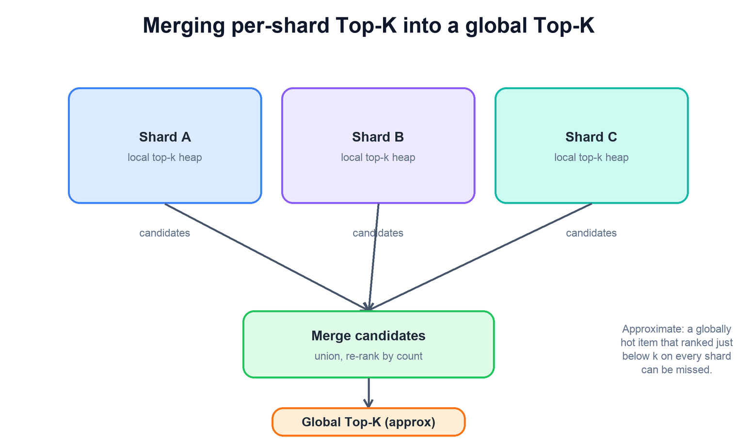
The Count-Min Sketches themselves merge cleanly: same dimensions and hash functions, add the grids cell by cell, and you get a sketch representing the union of all shards' events. The difficulty is the heaps. Each shard's heap only ever tracked the items that were heavy on that shard, so an item that was, say, the eleventh most popular on every shard — never quite making any local top ten — may be genuinely top ten globally yet appear in no shard's heap. Its identity was discarded locally before the merge could see it.

The practical merge therefore works on candidate sets: take the union of every shard's local top-k items, then re-rank that combined candidate list by global frequency — either by summing each candidate's per-shard estimates or by querying a merged sketch. To reduce the miss-an-item risk, shards usually track more than k locally (a top-2k or top-10k buffer), so an item that is moderately strong everywhere is more likely to survive into some shard's candidate list and reach the merge.

function global_top_k(shards, K):
  candidates = union(s.heap.items() for s in shards)   # local leaders only
  merged_cms = reduce(cms_merge, [s.cms for s in shards])
  scored = [(item, cms_estimate(merged_cms, item)) for item in candidates]
  return top_k_by_count(scored, K)                     # approximate — tail items can be missed

11. Accuracy Tradeoffs

There are at least two errors: estimated frequency may be inflated by hash collisions, and a true winner's identity may be missing from the candidate set. Larger width/depth reduces sketch error; larger candidate buffers mitigate discovery risk but do not prove arbitrary exact top-k recovery.

With width ceil(e/ε) and depth ceil(ln(1/δ)), a fixed item's estimate has an additive ε×total-weight upper bound with probability at least 1−δ under suitable independent hashing. This is not a guarantee that all adaptive queries always satisfy the bound; use an appropriate union bound or stronger analysis when reporting many items. Relative error is most relevant near the cutoff, where rankings are fragile.

Use the downloaded model to test the local-top-k counterexample and the non-underestimation invariant. For a production heavy-hitter contract, evaluate Space-Saving or Misra–Gries with stated bounds, retain more candidates, or do exact refinement from the replayable stream. Report frequency bounds and membership coverage separately.

12. Failure Modes

13. Tradeoffs and Alternatives

Worked example: a global winner missing from local top-1 lists

There are two shards, each keeping only its locally most frequent item.

Run a small, testable model

Download concepts.py. It uses only the Python 3.10+ standard library. From the directory where you saved it, run:

python3 concepts.py topk
python3 concepts.py test

The model constructs this counterexample and verifies both exact counts and the missing candidate; it also tests CMS non-underestimation.

The program contains deterministic assertions and failure traces. It is a learning model, not a production service: it does not implement network consensus, distributed durability, authentication, or third-party delivery. Read its contracts and try changing an input before extending it.

14. A 45-Minute Interview Plan

15. Common Mistakes

• Thinking CMS error is relative to the item. The bound is ε times the whole stream, N.
• Taking the average of the d cells. Every cell is an overcount; the minimum is the right estimate.
• Merging heaps by adding their counts. Items missing from a shard's heap are not zero there. Re-score candidates against a merged sketch.
• Decaying the sketch but not the heap. Stale leaders then block new items.
• Partitioning by item. A viral item overloads one worker. Partition randomly and merge.
• Computing the top-k on each read. Precompute and cache it; reads should be a key lookup.

16. Summary

A trending Top-K system finds the heaviest items in an unbounded stream without paying for the long tail. The design is a few interlocking decisions:

17. Check Yourself

1. You want overcounts of at most 0.1% of the stream with 99% confidence. What are w and d?
   Answer

   w = ⌈e/0.001⌉ = 2,719 and d = ⌈ln(100)⌉ = 5, so 13,595 counters. With 4-byte counters that is about 54 KB.

2. An item's cells hold 12, 15, and 9. What is its estimate, and what do you know about its true count?
   Answer

   The estimate is 9, the minimum. The true count is at most 9 (every cell is ≥ true), and with probability 1−δ it is at least 9 − εN.

3. Why can a Count-Min Sketch overcount but never undercount?
   Answer

   Each cell holds the item's own count plus counts of any items that collided there. Collisions only add, so every cell, and therefore the minimum, is ≥ the true count.

4. Two shards each keep a top-10 heap. Why can the merged top 10 be wrong?
   Answer

   An item ranked 11th on every shard appears in no heap, yet its global total may be top 10. Track a larger local buffer and re-score the union of candidates against a merged sketch.

5. You decay all sketch counters by half every hour but forget the heap. What goes wrong?
   Answer

   The heap's stored estimates stay at the old, larger values. New items, measured with decayed counts, rarely beat the heap minimum, so the list freezes on old leaders.

6. With N = 20.8 M events per hour and ε = 10⁻⁵, is the sketch accurate enough to rank an item seen 30,000 times? One seen 150 times?
   Answer

   The worst overcount is about 208. For 30,000 that is under 1%, so ranking is fine. For 150 the error can exceed the count itself, so the sketch cannot rank it.

18. Key Terms

Heavy hitter

An item whose frequency is a large share of the stream.

Count-Min Sketch

A matrix of shared frequency counters with one hash-selected cell per row. Increment all selected cells; estimate one item's count using the smallest selected counter. Collisions only add extra counts in an insertion-only, nonnegative stream. Example and limits above.

ε, δ

Error fraction of N and failure probability; set w and d.

N

Total number of events added to the sketch.

Min-heap

A tree whose root is the smallest element; keeps the current top k.

Tumbling window

Fixed, non-overlapping time buckets (e.g. each minute).

Sliding window

The last T time units, advanced as time moves on.

Exponential decay

Scaling old counts down so recent events weigh more.

Space-Saving

A heavy-hitters algorithm with m counters that replaces the minimum.

Misra-Gries

A deterministic heavy-hitters algorithm with k−1 counters.

Further reading

• Graham Cormode and S. Muthukrishnan, "An Improved Data Stream Summary: The Count-Min Sketch and its Applications," Journal of Algorithms, 2005.
• Ahmed Metwally, Divyakant Agrawal, Amr El Abbadi, "Efficient Computation of Frequent and Top-k Elements in Data Streams," ICDT 2005 (Space-Saving).
• Jayadev Misra and David Gries, "Finding Repeated Elements," Science of Computer Programming, 1982.
• Moses Charikar, Kevin Chen, Martin Farach-Colton, "Finding Frequent Items in Data Streams," ICALP 2002 (Count Sketch).
• Apache DataSketches documentation: frequent items sketch.